By Shengyu
TPC-H, as an OLAP benchmark, has been the subject of numerous optimization articles [1,2]. The following table shows the performance data of the TPCH 100GB test set in six different public cloud instance types:
| Specifications | 8c32g * 2 | 8c32g * 4 | 16c64g * 2 | 16c64g * 3 | 16c64g * 4 | 16c64g * 6 |
|---|---|---|---|---|---|---|
| Total Time Required (Seconds) | 99.82 | 48.55 | 50.31 | 33.00 | 25.54 | 20.56 |
The following table shows the performance data of the TPCH 1TB test set in three different public cloud instance types:
| Specifications | 3*16C128GB | 4*16C128GB | 6*16C128GB |
|---|---|---|---|
| Total Time Required (Seconds) | 508.76 | 408.45 | 233.93 |
In the previous article, we introduced the PolarDB-X column-oriented storage query engine [3]. While pursuing TPC-H scores is not the ultimate goal, results that are far from satisfactory are also unacceptable. During our research, we found that most database vendors generally publish testing procedures and results on their official websites, but they rarely provide detailed execution plans. The reason is probably simple: for optimizers, especially with join reordering, TPC-H is considered a relatively simple benchmark [4].
This situation led us to spend a considerable amount of time repeatedly setting up database environments, generating TPC-H data, importing TPC-H data, analyzing TPC-H execution plans, and producing research reports across various databases. To reduce workload, we will provide an official interpretation of the PolarDB-X TPC-H 1T column-oriented execution plan in this article. Points to note:
• The execution plan is based on the explain analyze output from polardb-2.4.0_5.4.19-20240527_xcluster5.4.19-20240527, and the corresponding execution plan text has been open-sourced [5]. Future versions may vary, so please refer to the open-source text.
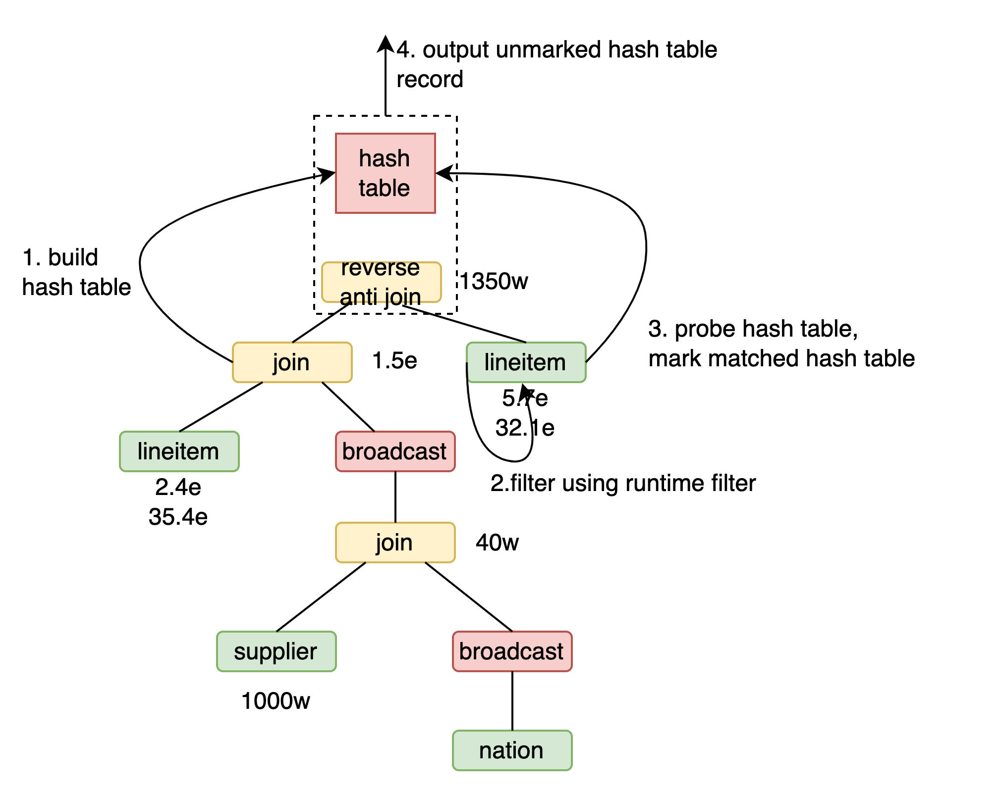
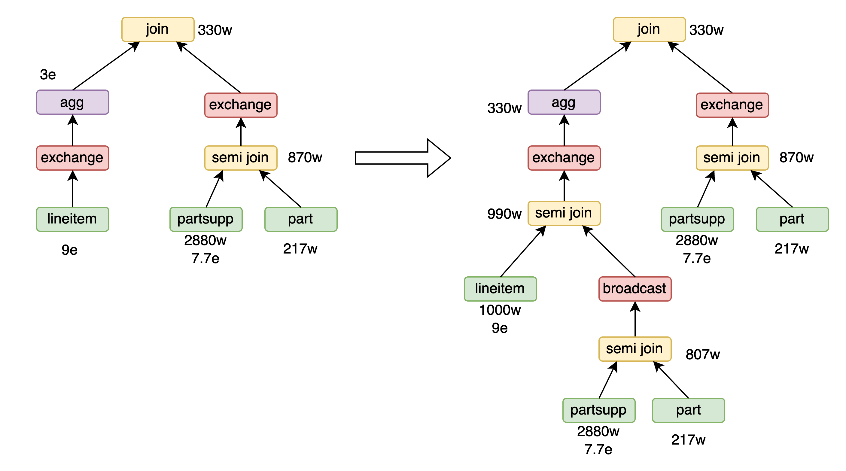
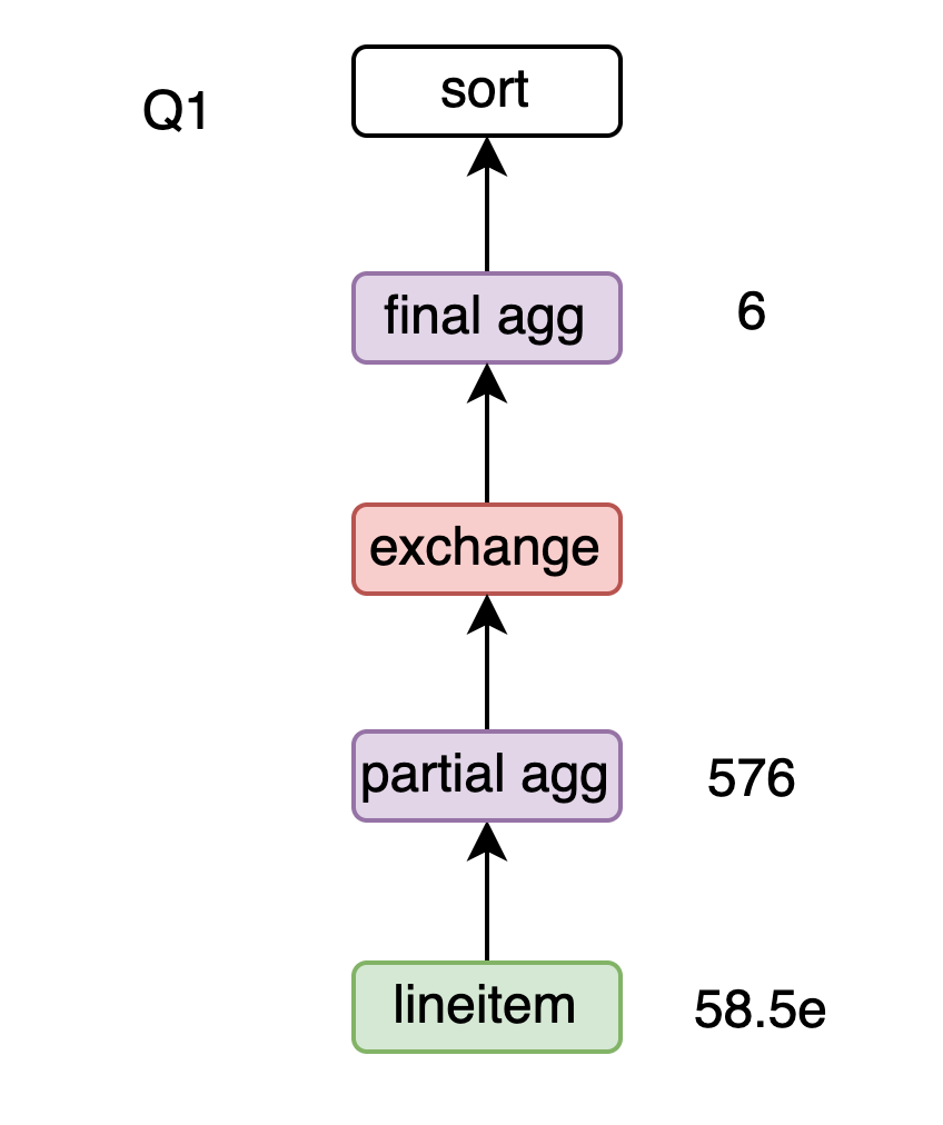
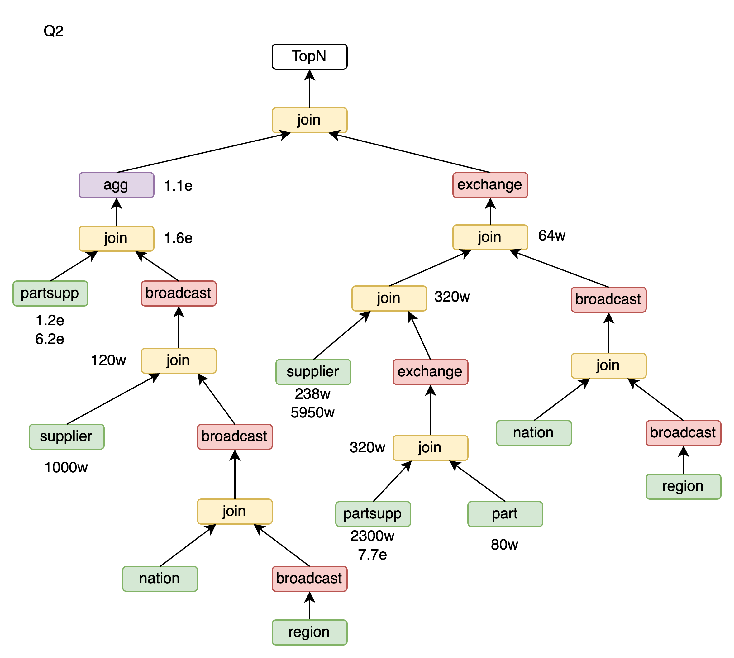
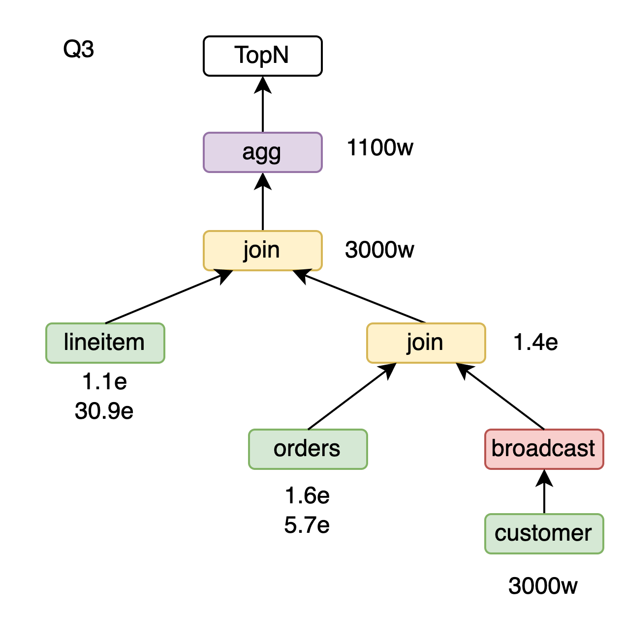
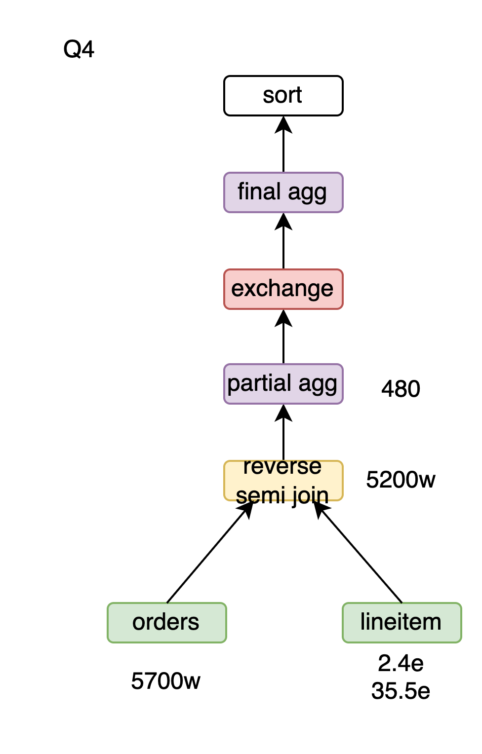
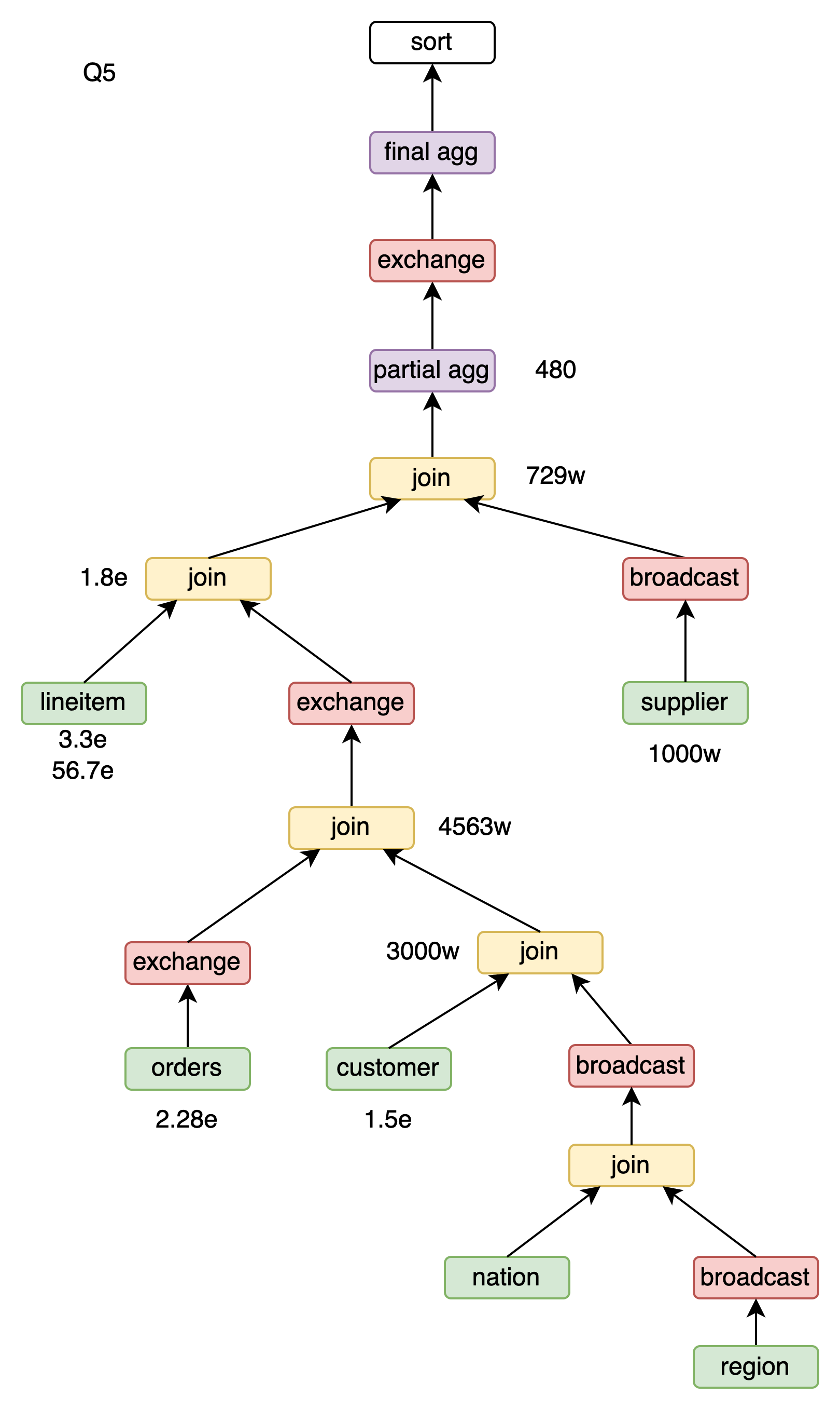
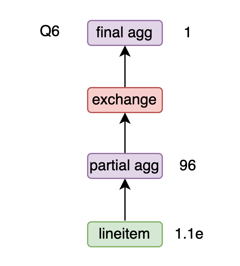
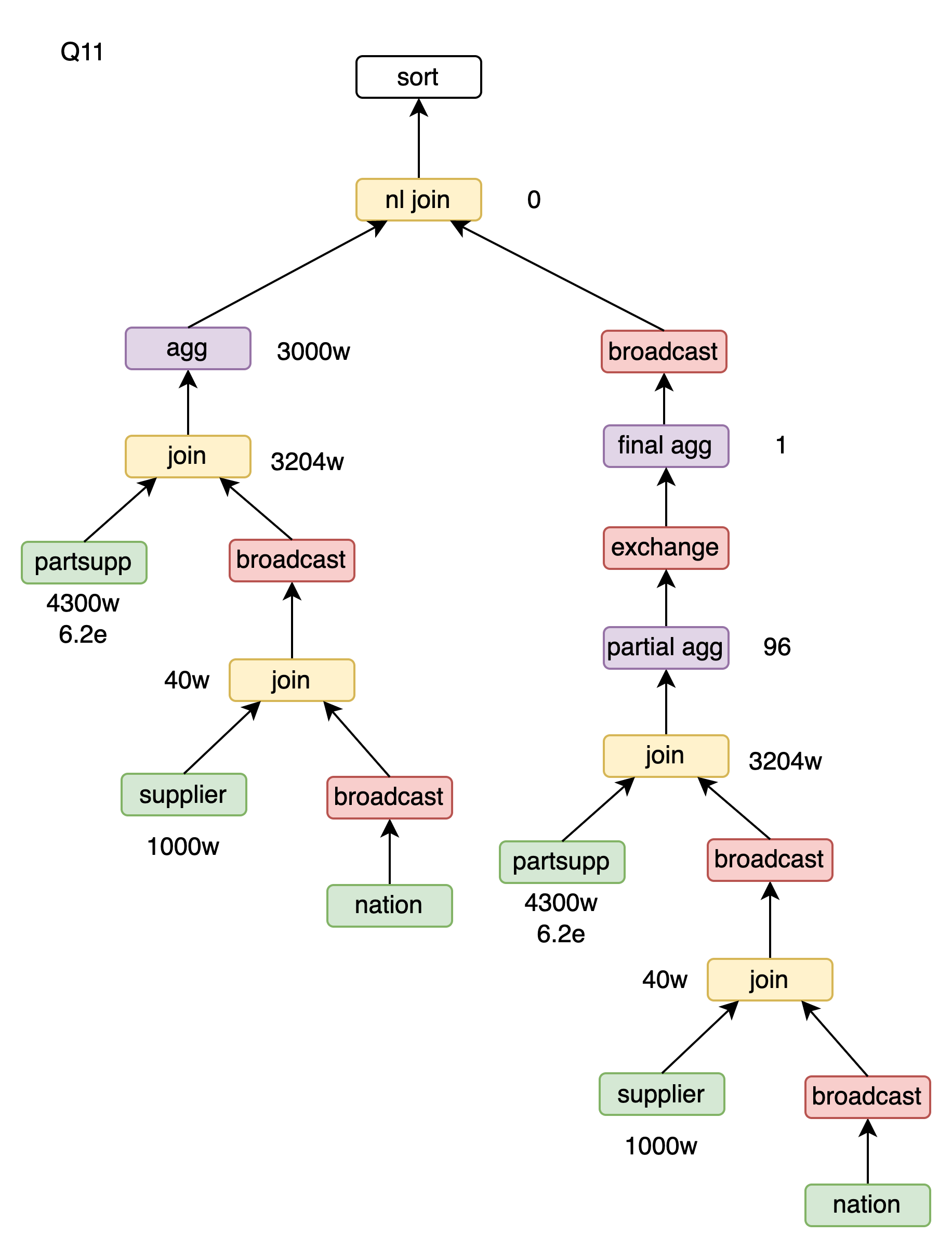
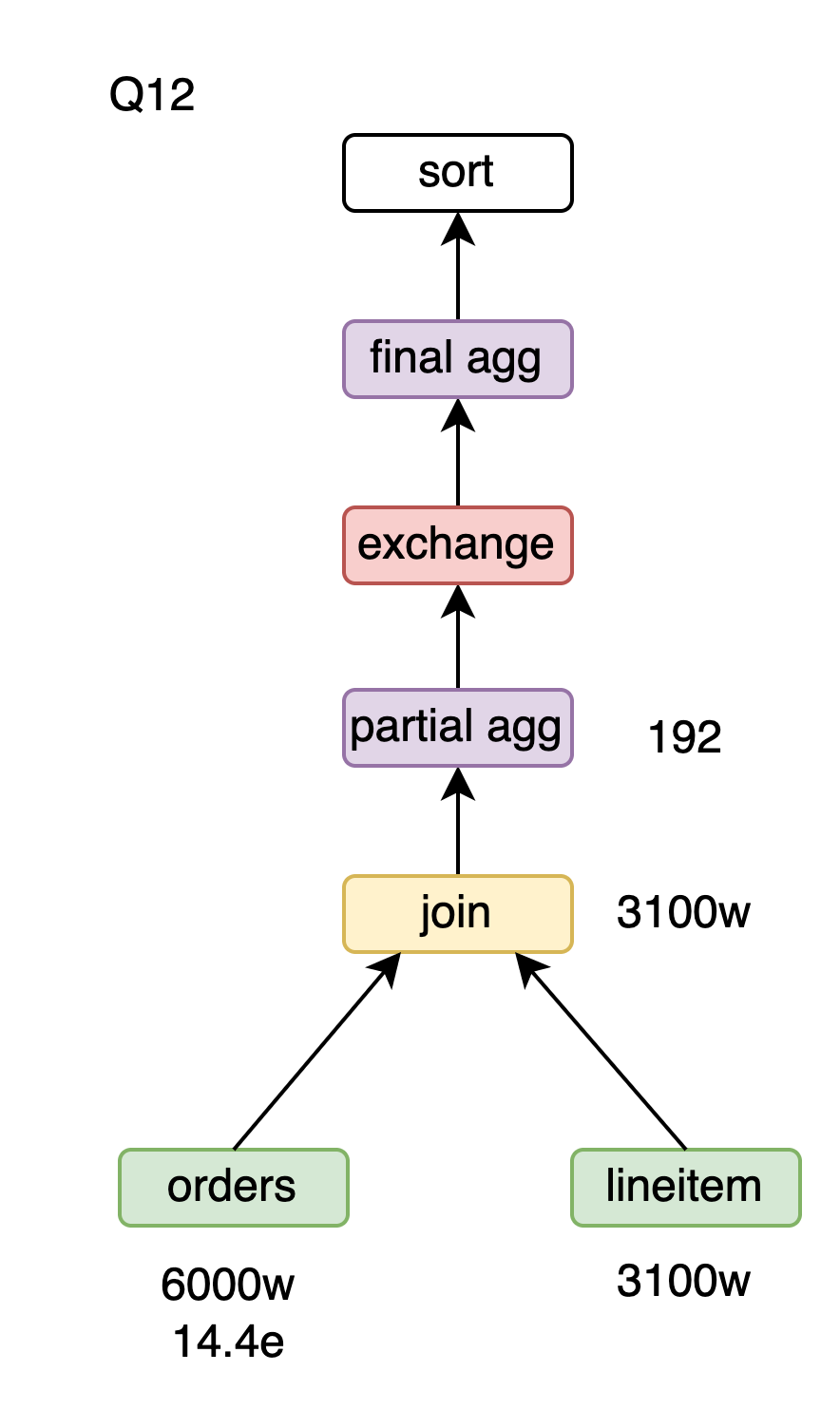
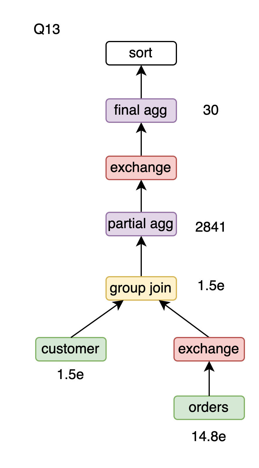
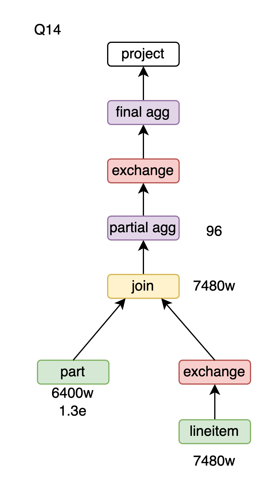
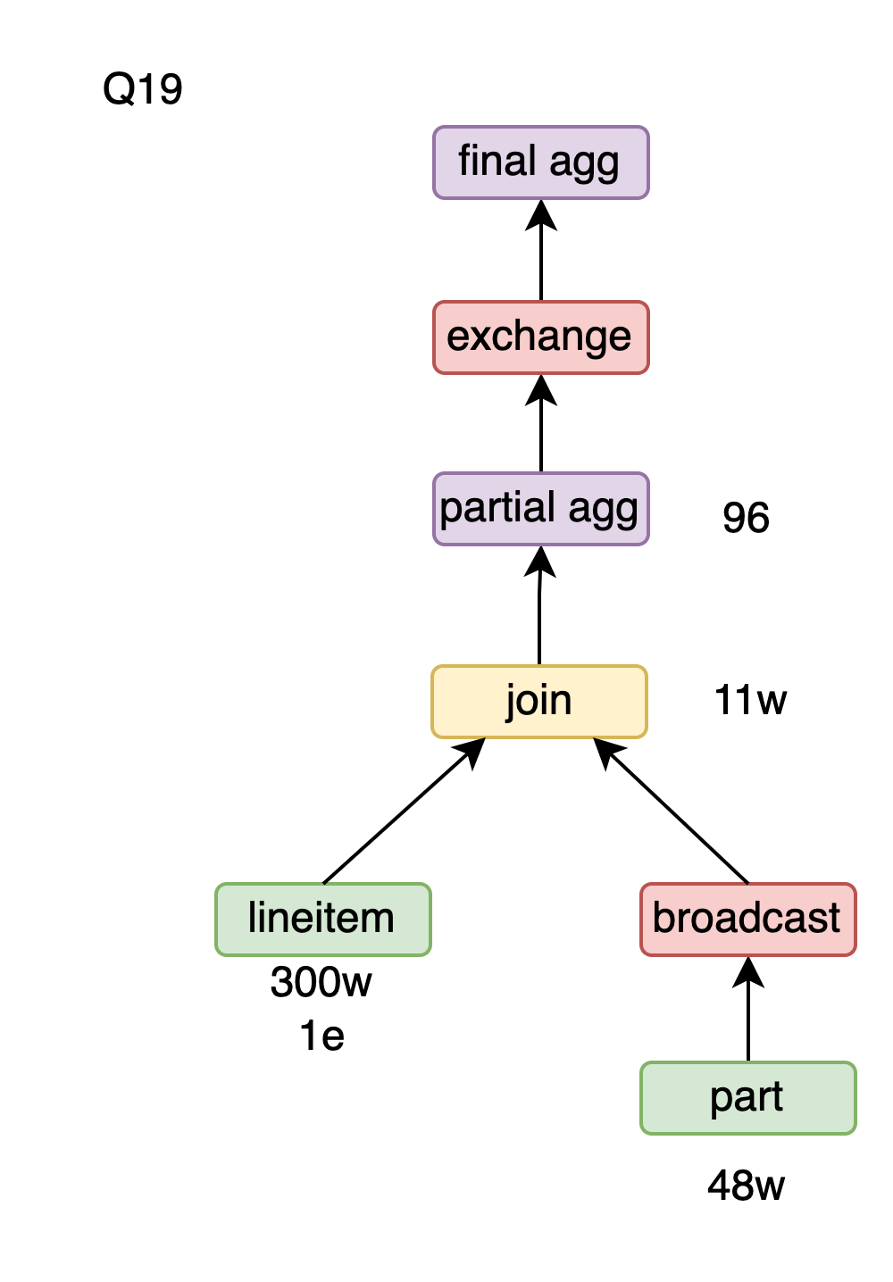
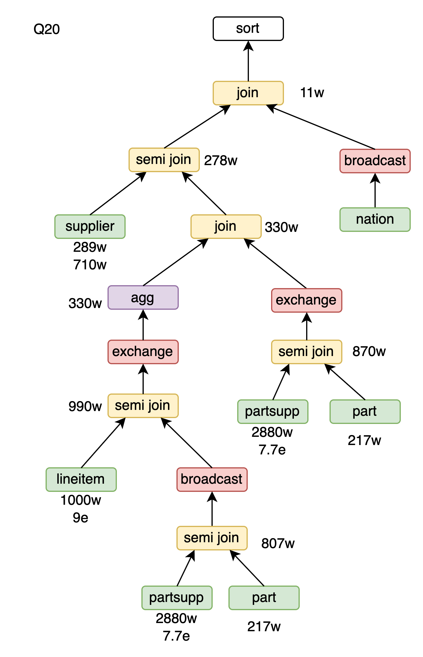
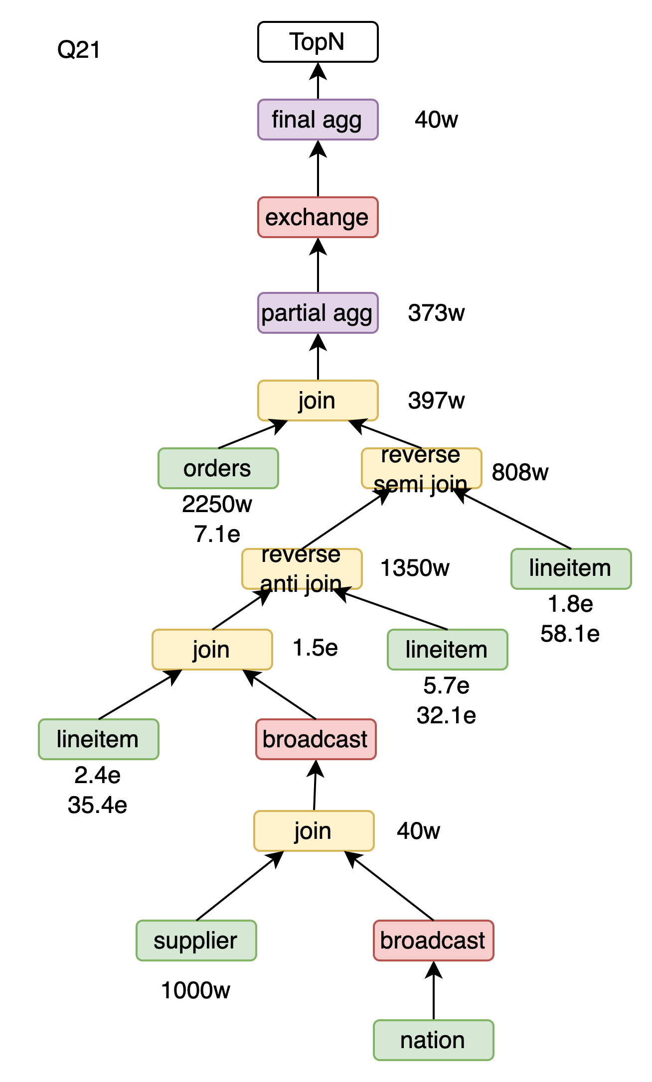
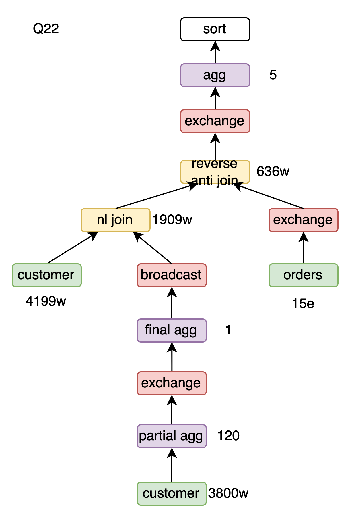
• The numbers in the figure represent the number of output rows for the respective operators. If there are two rows of numbers, the second row indicates the number of rows filtered by the runtime filter.
• Unless specified as reverse, hash joins by default have the right child building the hash table, and the left child probing it.
• For simplicity, project operators are omitted from the figures.
• TPC-H usually includes order by limit, which does not involve much computation; at the root of the tree, this is simplified into a single operator.
The PolarDB-X optimizer [6] includes RBO and CBO, with the CBO being a standard Cascade style Top-Down optimizer. The cardinality estimation is based on a traditional model that assumes independence. Statistics [7] include histograms, TopN, and NDV. The optimizer architecture of the current version is as follows:

In PolarDB-X, column-oriented storage is an index form, and the optimizer automatically uses columnar indexes in the way it would select indexes. When the optimal single-server physical execution plan B optimized by the CBO is an AP query and columnar indexes can be used, it will enter the columnar optimizer:
Both the columnar optimizer and the MPP optimizer generate distributed execution plans. The difference is that the MPP optimizer inserts the shuffle operator into the physical execution plan B to generate distributed execution plans, while the columnar optimizer generates the optimal distributed execution plan based on the logical execution plan A.
The reason the MPP optimizer optimizes based on execution plan B is that the performance of row-based queries is primarily determined by the DN, and data distribution is not critical. In addition, keeping the same execution path as the single-server execution plan avoids the situation where MPP execution could be slower due to differences in the execution plan.
The columnar optimizer optimizes based on execution plan A because data redistribution, which is a key factor in columnar query speed, must be considered during join reordering.
The compute nodes of PolarDB-X follow an MPP architecture, and the executor schedules the same data to the same compute node for processing, facilitating cache reuse. Scheduling granularity can be at the file or partition level. For partition-level scheduling, data with the same partition key is guaranteed to land on the same compute node, which is referred to as partition wise. This scheduling is related to the partitioning method of the table and can be recognized by the optimizer as a partition-wise attribute of a table, used to minimize data redistribution.
One compute node is assigned to each partition, which is a classic Balls into Bins problem. To reduce the maximum load, when random scheduling is uneven, the "two choices" approach [8] is re-employed, trading twice the space for an exponential decrease in skew ratio.
The columnar CBO of PolarDB-X exhaustively enumerates all possible join orders [9] and provides capabilities such as semijoin-join swapping and agg-join swapping to ensure a reasonable join order. Given that the search space for the columnar CBO is the result of the single-serv CBO✖MPP CBO, to prevent the optimizer from being too time-consuming, join reordering is not performed when there are more than 10 tables. The use of runtime filters significantly improves join performance.
Runtime filters in PolarDB-X are not generated by the optimizer, and the cost model does not take into account the filtering effect of runtime filters.
Runtime filters are adaptively built by the executor, so only during actual execution can it be known if a runtime filter is used; this information cannot be shown during explain analyze.
For Join operators, PolarDB-X supports Hash Join, Sort Merge Join, BKA Join, and Nested Loop Join. The row-based optimizer selects the operator with the lowest cost among these; the columnar optimizer prefers Hash Join and falls back to Nested Loop Join if Hash Join cannot be used.
For Agg operators, PolarDB-X supports Hash Agg and Sort Agg. The row-based optimizer chooses the least costly operator, while the columnar optimizer uses only Hash Agg.
For Window operators, PolarDB-X supports Hash Window and Sort Window.
Since Hash Window cannot cover all scenarios, the columnar optimizer, like the row-based optimizer, will choose the less costly physical operator between Hash Window and Sort Window.
All improvements and corresponding queries are listed as follows:
| Improvements | Queries that can be applied |
|---|---|
| Partition wise | Q2, Q3, Q4, Q9, Q10, Q12, Q13, Q14, Q16, Q18, Q21 |
| Column pruning | Q1-Q22 |
| Constant folding | Q1, Q4, Q5, Q6, Q14, Q15, Q19, Q20 |
| Two-phase agg | Q1, Q4, Q5, Q6, Q7, Q8, Q9, Q11, Q12, Q13, Q14, Q15, Q16, Q17, Q19, Q21, Q22 |
| Cardinality estimation | Q9, Q13 |
| Reverse semi hash join | Q4, Q21 |
| Reverse anti hash join | Q21, Q22 |
| Join-Agg to Join-Agg-Semijoin | Q20 |
| Group join | Q13 |
| Hash window | Q17 |
Taking Q3 as an example, lineitem is sharded by l_orderkey, orders is sharded by o_orderkey, and customer is sharded by c_custkey.
select
    1
from
    customer,
    orders,
    lineitem
where
    c_custkey = o_custkey
    and l_orderkey = o_orderkey
group by
    l_orderkey,
    o_orderdate,
o_shippriority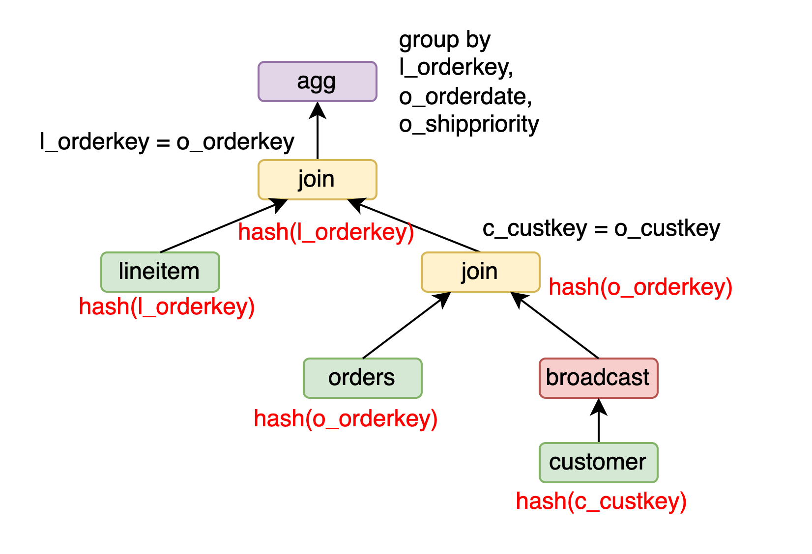
For the orders join customer, if customer is broadcasted, the orders join customer can maintain the sharding attribute of o_orderkey. Further, for lineitem join (orders join customer), since lineitem has a sharding attribute of l_orderkey and orders join customer has a sharding attribute of o_orderkey, a partition-wise join can be performed, maintaining the sharding attribute of l_orderkey. For the final group by l_orderkey, o_orderdate, and o_shippriority, because the input maintains the sharding attribute of l_orderkey, a partition-wise agg can be performed.
The broadcast join of PolarDB-X is implemented based on the passThroughTrait of Calcite. For example, when broadcasting the right table, the distribution attributes of the join and the left child is set to any, while the distribution attributes of the right child is set to broadcast.
void columnarBroadCastRight(Join join, RelNode leftChild, RelNode rightChild) {
    join.Distribution = ANY;
    leftChild.Distribution = ANY;
    rightChild.Distribution = BROADCAST;
    return;
}
If the distribution attributes of the right child is broadcast, the passThroughTrait will propagate the required join distribution attributes to the left child, thereby passing them down until they reach the columnar index.
void passThroughTrait(
    Distribution required, Join join, RelNode leftChild, RelNode rightChild) {
    RelDistribution distribution = required.Distribution;
    if (rightChild.Distribution == BROADCAST) {
        for (int key : required.getKeys()) {
            if (key >= leftInputFieldCount) {
                return;
            }
        }
        join.Distribution = required;
        leftChild.Distribution = required;
    }
}
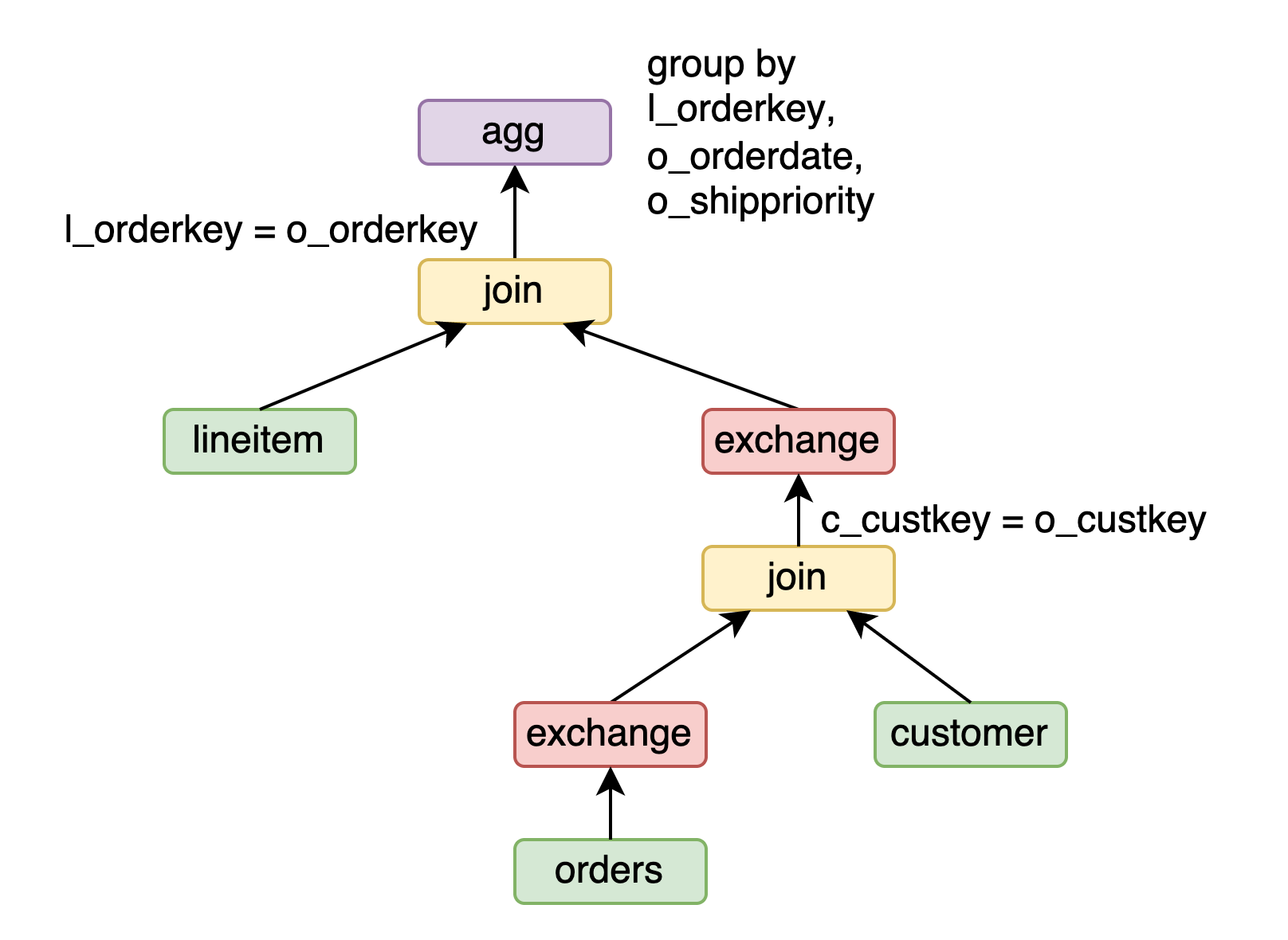
Besides broadcast, exchange can also be used. For instance, in Q3, orders can be exchanged by o_custkey to obtain the sharding attribute of o_custkey. Since customer has a sharding attribute of c_custkey, orders join customer can perform a partition-wise join. Then, orders join customer can be exchanged by o_orderkey, allowing lineitem join (orders join customer) to perform a partition-wise join.
Since this execution plan requires two exchanges, which is more costly than the broadcast plan, the CBO does not choose it.
The issue with columnarBroadcastRight and passThroughTrait working together is that a broadcast join might pass through all output columns, leading to a dramatic increase in the search space. Therefore, unnecessary broadcast joins must be pruned early.
The pruning logic is as follows: For A join B, A join broadcast(B) can always be represented as shuffle(shuffle(A) join shuffle(B)). If the cost of broadcast(B) is greater than the cost of shuffle(A) + shuffle(B) + shuffle(A join B), the optimizer can avoid generating the redundant A join broadcast(B), and thus, there is no need to pass through any column of A.
To reduce the shuffle cost in large-scale data processing tasks, it is necessary to prune columns using a project operator before the shuffle operation, thereby reducing redundant columns. Join operations often introduce redundant columns, which can increase the amount of data shuffled and lead to performance degradation. The NET cost formula for the shuffle operator is designed as NET_COST = rowSize * rowCount / NET_BUFFER_SIZE, where rowSize refers to the amount of data per row. Clearly, a larger rowSize directly increases the shuffle cost, so the CBO naturally chooses an execution plan with column pruning.
public RelOptCost computeSelfCost() {
    double rowCount = getRowCount();
    long rowSize = estimateRowSize(getInput().getRowType());
    if (distribution == BROADCAST) {
        rowCount = rowCount * parallelism;
    }
    cpuCost=...;
    netCost = rowSize * rowCount / NET_BUFFER_SIZE);
    return costFactory.makeCost(rowCount, cpuCost, 0, 0,
                                Math.ceil(netCost);
}
The key points for implementing column pruning are:
Constant folding allows the optimizer to calculate constants that can be directly calculated in advance. For example, in Q1, the filter condition l_shipdate <= '1998-12-01' - interval '118' day would be optimized to l_shipdate <= '1998-08-05'.
Since constant folding is applied only once and does not have strict performance requirements, it can directly call the computation interface of the scalar function. It is important to note that the parser of PolarDB-X parameterizes constants to facilitate plan cache matching. The filter condition of Q1 is parameterized to l_shipdate <=? - interval ? day. After constant folding to l_shipdate <= '1998-08-05', the execution plan cannot be reused, making constant folding incompatible with plan caching. By default, the columnar plan cache is disabled, and constant folding is enabled. If the columnar plan cache is enabled, constant folding will automatically be disabled.
For Q1, the group by l_returnflag, l_linestatus needs to be split into two phases to avoid shuffling a large amount of data. First, a partial agg (group by l_returnflag, l_linestatus) is performed at the shard level, followed by a global agg (group by l_returnflag, l_linestatus). This reduces the shuffle data volume from 585 million rows to 576 rows. However, if the agg itself produces a large number of results, the two-phase agg might not reduce the shuffle volume and could introduce redundant agg calculations. Therefore, it is necessary to use cardinality estimation to determine if the two-phase agg is beneficial. Since the partial agg is performed at the shard level, there can be an amplification of the result set. The formula for cardinality estimation needs to be adjusted as follows: rows is the total number of input rows, and bins is the estimated row count for the agg. Considering each shard, there are 
rows of data per shard, with bins different groups. This is also a Balls into Bins problem, and the rowcount is estimated as follows:

For x join y on x.a = y.b and x.c = y.d, the calculation formula of cardinality estimation is:
x.rows∗y.rows/max(max(ndv(x.a),ndv(y.b)),max(ndv(x.c),ndv(y.d)))
In Q9, the join condition ps_suppkey = l_suppkey and ps_partkey = l_partkey involves a composite primary key in partsupp. The cardinality estimation for the join should be modified to:
x.rows∗y.rows/max(ndv(x.a,x.c),ndv(y.b,y.d))
For the filter condition p_name like '%goldenrod%' in Q9, there is no specific handling, and a heuristic approach is used, setting the filterability to 5%. In Q13, the group by c_count where c_count is the result of count(o_orderkey) group by c_custkey cannot have its ndv estimated. A heuristic is used, setting ndv to 100.
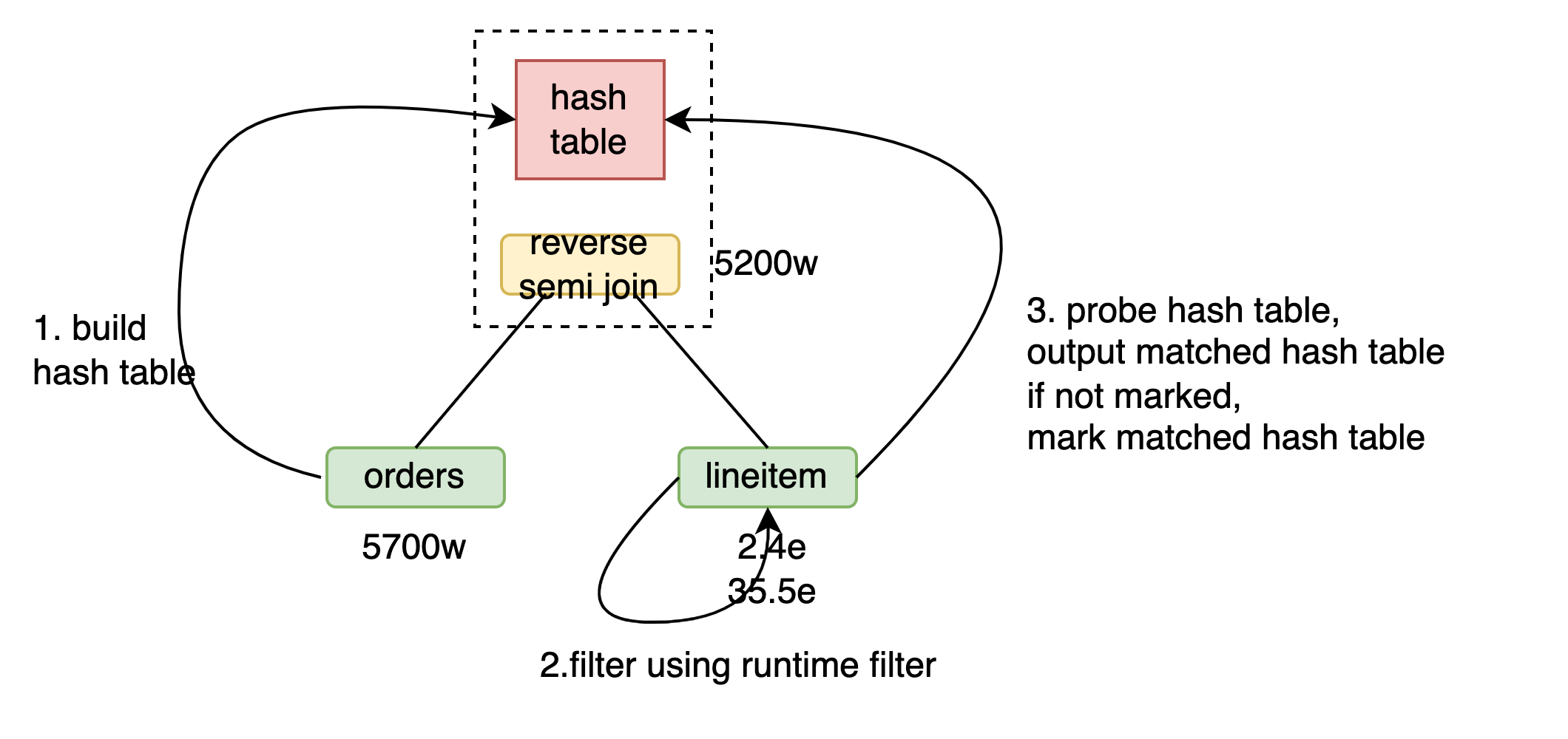
In Q4, the EXISTS subquery is converted to a semi join, resulting in orders semi join lineitem. The process for orders semi hash join lineitem is as follows:
For orders reverse semi hash join lineitem, the process is:
Since probing a hash table is much more efficient than building one, the reverse semi hash join is more efficient in this scenario.

For B semi hash join A, it is clear that a runtime filter can be built using A to filter elements of B.
For B reverse semi hash join A, a runtime filter can also be used, built using B to filter elements of A.
Here is the proof:
Let the result set of A after applying the runtime filter be C. To prove that B reverse semi hash join A ⇔ B reverse semi hash join C, we need to show that B∩A⇔B∩C. Since C⊂A, the reverse direction is clearly true. Considering the forward direction, for ∀x, if x ∈ B ∩ A, by the nature of the runtime filter, x ∈ B implies filterB(x) = true, so x ∈ C. Therefore, ∀x, x ∈ B ∩ A ⇒ x ∈ B ∩ C.
The process for orders reverse semi hash join lineitem with a runtime filter is:
Since the efficiency of probing a runtime filter is much higher than probing a hash table, the introduction of a runtime filter in this scenario results in higher efficiency.
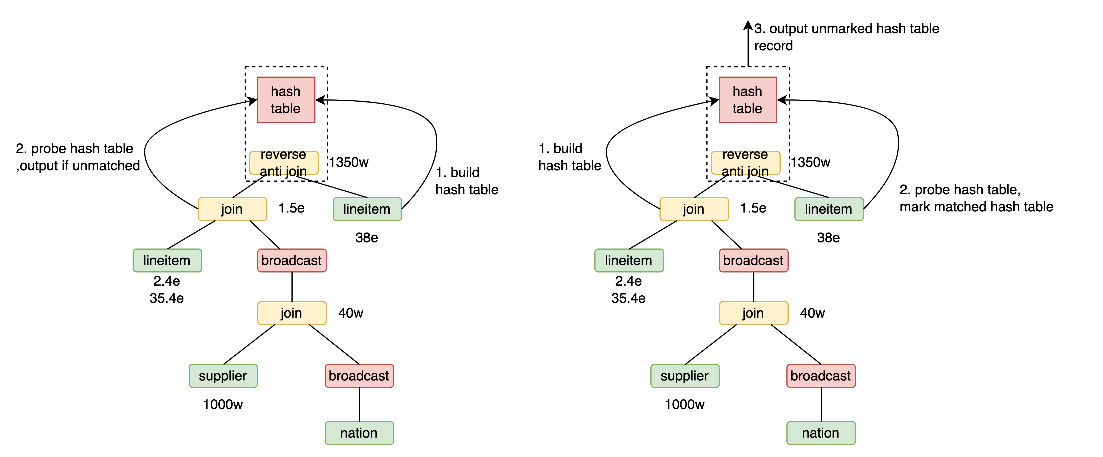
In Q21, the NOT EXISTS subquery is converted to an anti join, resulting in xx anti join lineitem, where xx is the result of joining the lineitem, supplier, and nation tables. The process for xx anti hash join lineitem is as follows:
For xx reverse anti hash join lineitem, the process is:
Since probing a hash table is much more efficient than building one, the reverse anti hash join is more efficient in this scenario.
For B reverse anti hash join A, a runtime filter based on B can be used to filter elements of A. Here is the proof: Let the filtered result set be C. To prove that B reverse anti hash join A ⇔ B reverse anti hash join C, we need to show that
BA⇔BC. Since C ⊂ A, the forward direction is clearly true. For the reverse direction, for ∀x, if x ∈ B C, then x ∈ B and x ∉ C. By the nature of the runtime filter, x ∈ B implies filter_B(x) = true, or x ∉ C implies x ∉ A or filter_B(x) = false. Therefore, x ∈ B C implies filter_B(x) = true and (x ∉ A or filter_B(x) = false), which means x ∉ A. Thus, for ∀x, x ∈ B C ⇒ x ∈ B A.
The process for xx reverse anti hash join lineitem with a runtime filter is:
Since the efficiency of probing a runtime filter is much higher than probing a hash table, the introduction of a runtime filter in this scenario results in higher efficiency.
Currently, the runtime filter of PolarDB-X cannot penetrate shuffle operations on the probe side of a join. This limitation negatively impacts the performance of Q20 queries: a large number of redundant results are calculated from the lineitem table during aggregation, and using a runtime filter before the aggregation to eliminate these redundancies could improve performance. However, the shuffle between the lineitem table and the agg operation prevents the runtime filter from being pushed down. To address this issue, we introduced a CBO rule: duplicate the right child node of the join and perform a semi join with the input of the aggregation, effectively serving as a runtime filter.
Group joins have overly strict limitations and can have negative effects, leading to limited practical application. For more details, please refer to this article [10]. PolarDB-X currently restricts group joins as follows:
The global uniqueness requirement is primarily to avoid the problem of intermediate result set amplification caused by group joins. For Q13, a group join can be applied.
select
    c_custkey,
    count(o_orderkey) as c_count
from
    customer
    left outer join orders on c_custkey = o_custkey
    and o_comment not like '%special%packages%'
group by
c_custkey
Execution process of group join
Converting the subquery in Q17 to a window function saves one scan of the lineitem table, and further, a hash window can be used. Due to differences in parallelism, hash windows are more efficient than sort windows in PolarDB-X. To convert a window to a hash window, three conditions must be met:
This article provides an official, detailed explanation of the design points in PolarDB-X's TPC-H columnar execution plan. These points not only cover the principles of various optimizations but also provide relevant proofs and code implementations, aiming to help readers gain a deeper understanding of PolarDB-X's columnar optimizer. In the next article, we will explore the hybrid row-column execution plans of PolarDB-X.
[1] https://www.vldb.org/pvldb/vol13/p1206-dreseler.pdf
[2] https://homepages.cwi.nl/~boncz/snb-challenge/chokepoints-tpctc.pdf
[3] https://zhuanlan.zhihu.com/p/701718682
[4] https://cedardb.com/docs/example_datasets/job/
[5] https://github.com/polardb/polardbx-sql/blob/main/polardbx-optimizer/src/test/resources/com/alibaba/polardbx/planner/oss/Tpch1TTest.yml
[6] https://zhuanlan.zhihu.com/p/336084031
[7] https://zhuanlan.zhihu.com/p/580127024
[8] https://www.ic.unicamp.br/~celio/peer2peer/math/mitzenmacher-power-of-two.pdf
[9] https://zhuanlan.zhihu.com/p/470139328
[10] https://vldb.org/pvldb/vol14/p2383-fent.pdf
TPCH execution plan summary
Q1
Q2
Q3
Q4
Q5
Q6
Q7
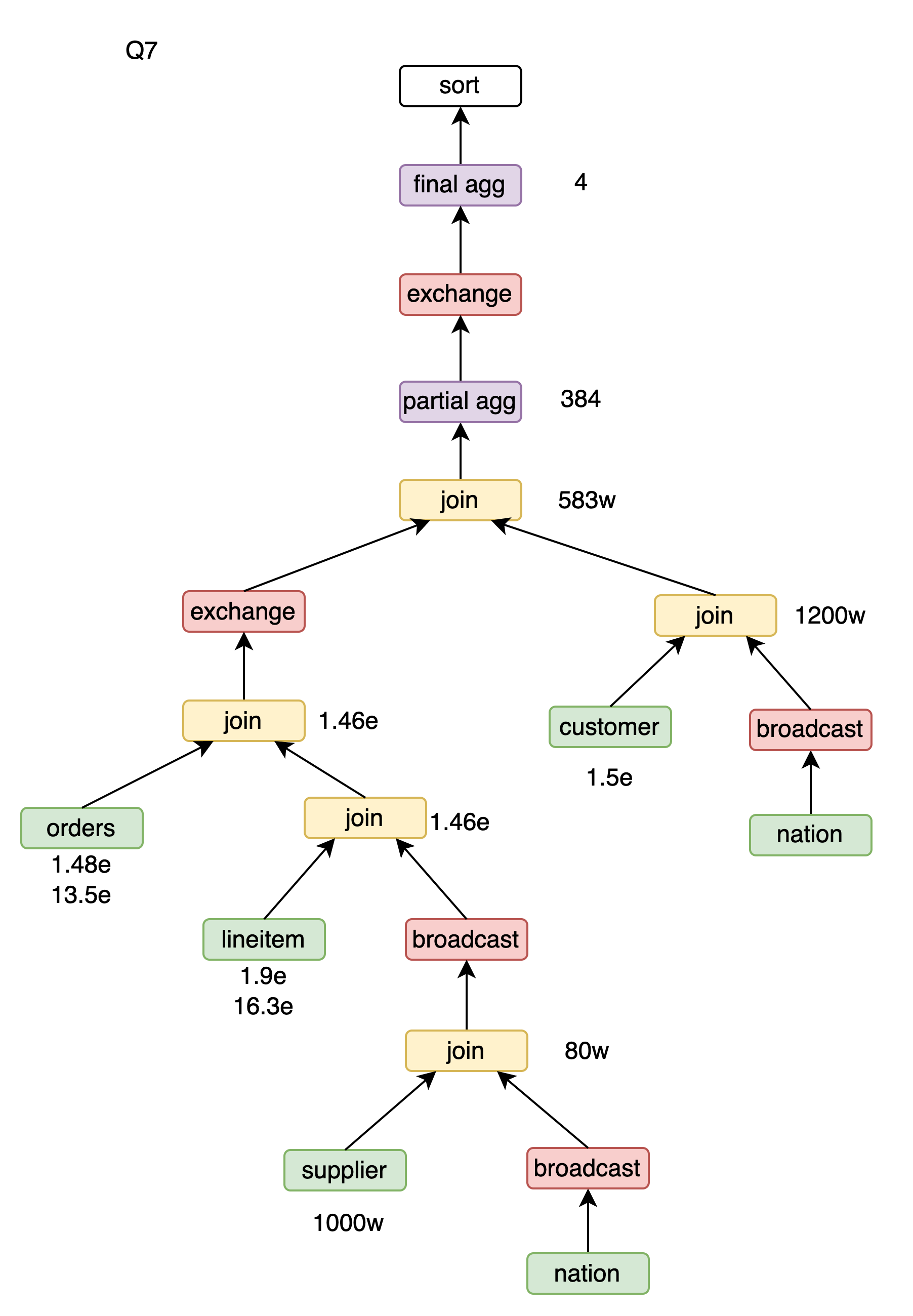
Q8
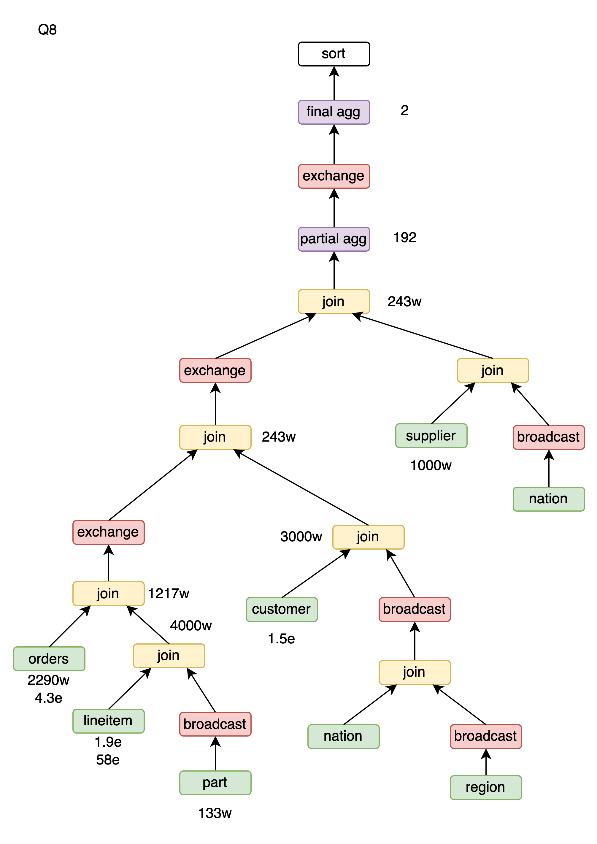
Q9
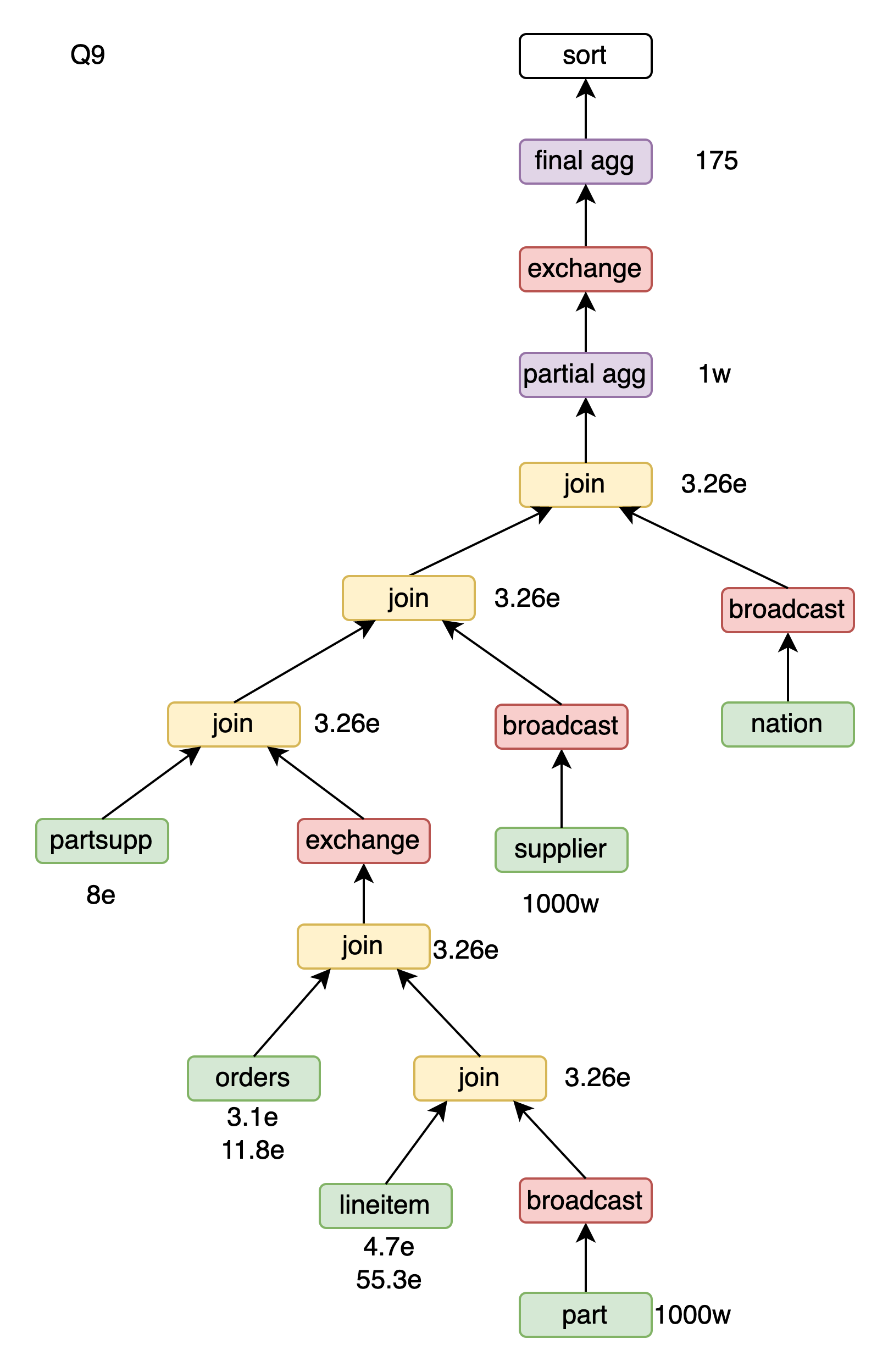
Q10
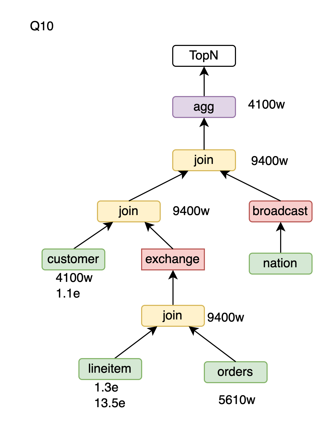
Q11
Q12
Q13
Q14
Q15
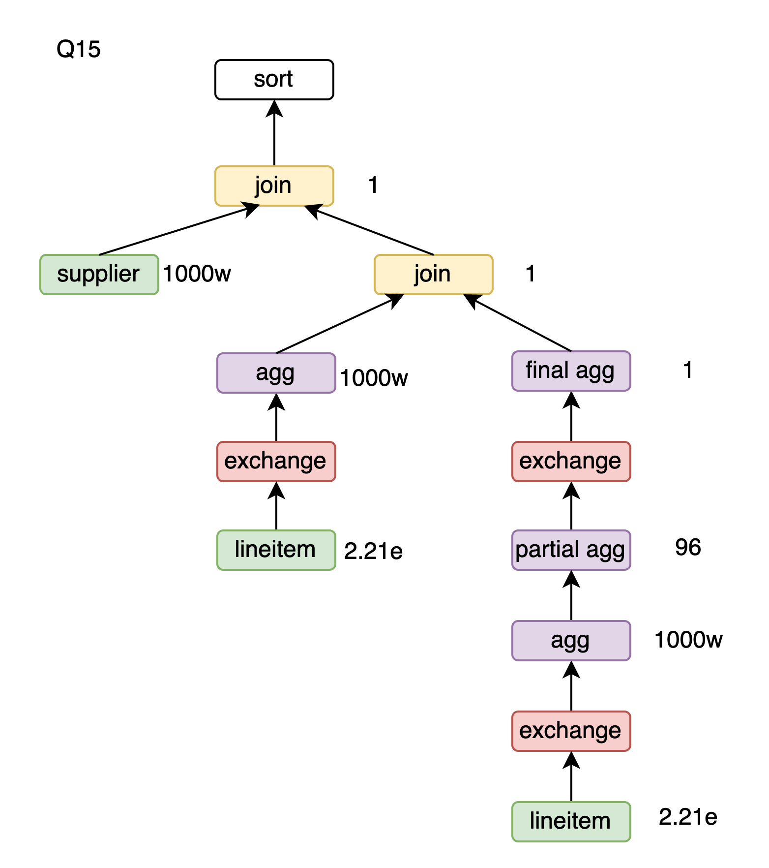
Q16
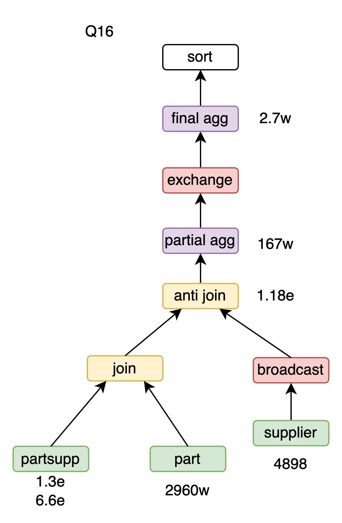
Q17
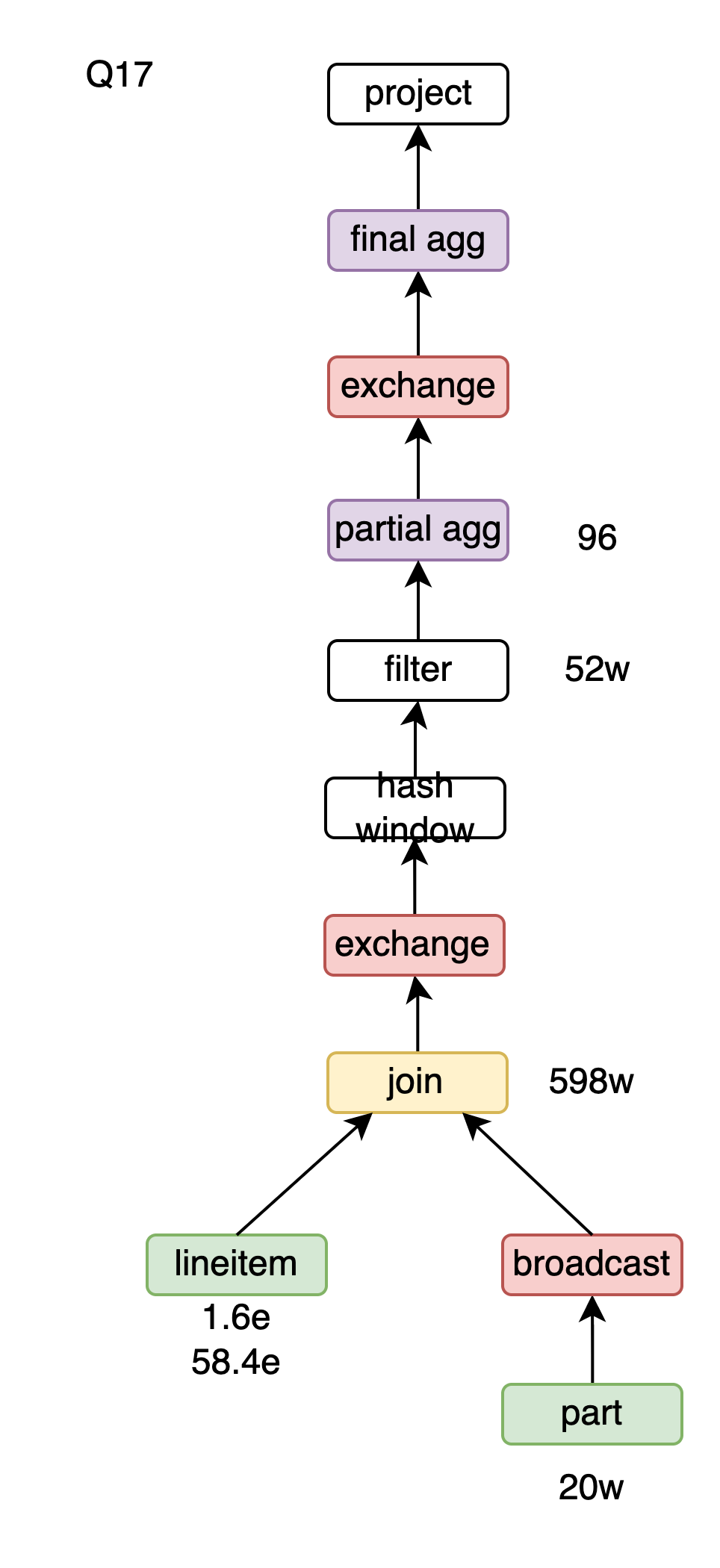
Q18
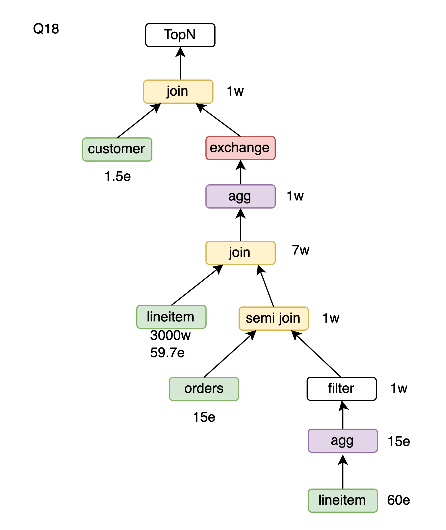
Q19
Q20
Q21
Q22
Core Technology of PolarDB-X Storage Engine | Lizard B+tree Optimization
PolarDB-X Disaster Recovery Capabilities: Cross-AZ, Cross-Region, and Cross-Cloud
ApsaraDB - October 16, 2024
ApsaraDB - April 10, 2024
ApsaraDB - June 19, 2024
ApsaraDB - March 26, 2025
ApsaraDB - November 24, 2025
ApsaraDB - October 16, 2024
 PolarDB for PostgreSQL
Alibaba Cloud PolarDB for PostgreSQL is an in-house relational database service 100% compatible with PostgreSQL and highly compatible with the Oracle syntax.
Learn More PolarDB for Xscale
Alibaba Cloud PolarDB for Xscale (PolarDB-X) is a cloud-native high-performance distributed database service independently developed by Alibaba Cloud.
Learn More PolarDB for MySQL
Alibaba Cloud PolarDB for MySQL is a cloud-native relational database service 100% compatible with MySQL.
Learn More Database for FinTech Solution
Leverage cloud-native database solutions dedicated for FinTech.
Learn MoreMore Posts by ApsaraDB