This topic describes how to build a streaming data lakehouse using Realtime Compute for Apache Flink, Paimon, and StarRocks.
Background information
As businesses become more digital, the demand for timely data grows. Traditional offline data warehouses follow a clear methodology. They use scheduled offline jobs to merge new changes from the previous period into a hierarchical warehouse that includes the Operational Data Store (ODS), Data Warehouse Detail (DWD), Data Warehouse Summary (DWS), and Application Data Store (ADS) layers. However, this approach has two major problems: high latency and high cost. Offline jobs typically run only once per hour or even once per day. This means data consumers can only see data from the previous hour or day. Additionally, data updates often overwrite entire partitions. This process is inefficient because it requires rereading all original data in the partition to merge it with new changes.
You can build a streaming data lakehouse using Realtime Compute for Apache Flink and Paimon to solve the problems of traditional offline data warehouses. The real-time computing capabilities of Flink allow data to flow between data warehouse layers in real time. The efficient update capability of Paimon allows data changes to be delivered to downstream consumers with minute-level latency. Therefore, a streaming data lakehouse has advantages in both latency and cost.
For more information about the features of Paimon, see Features and the Apache Paimon official website.
Architecture and benefits
Architecture
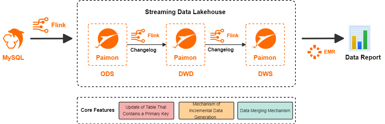
Realtime Compute for Apache Flink is a powerful stream processing engine that supports the efficient processing of large amounts of real-time data. Paimon is a unified lake storage format for stream and batch processing that supports high-throughput updates and low-latency queries. Paimon is deeply integrated with Flink to provide an integrated streaming data lakehouse solution. The following figure shows the architecture of a streaming data lakehouse built with Flink and Paimon:
Flink writes data from a data source to Paimon to form the ODS layer.
Flink subscribes to the changelog of the ODS layer, processes the data, and then writes it back to Paimon to form the DWD layer.
Flink subscribes to the changelog of the DWD layer, processes the data, and then writes it back to Paimon to form the DWS layer.
Finally, StarRocks in E-MapReduce reads the Paimon external table for application queries.
Benefits
This solution provides the following benefits:
Each layer of Paimon can deliver changes to downstream consumers with minute-level latency. This reduces the latency of traditional offline data warehouses from hours or even days to minutes.
Each layer of Paimon can directly accept change data without overwriting partitions. This greatly reduces the cost of data updates and corrections in traditional offline data warehouses. It also solves the problem of data at intermediate layers being difficult to query, update, and correct.
The model is unified and the architecture is simplified. The logic of the extract, transform, and load (ETL) pipeline is implemented using Flink SQL. Data at the ODS, DWD, and DWS layers is uniformly stored in Paimon. This reduces architectural complexity and improves data processing efficiency.
This solution relies on three core capabilities of Paimon. The following table provides details.
Paimon core capability | Details |
Primary key table updates | Paimon uses a Log-Structured Merge-tree (LSM Tree) data structure at the underlying layer to achieve efficient data updates. For more information about Paimon primary key tables and underlying data structures, see Primary Key Table and File Layouts. |
Incremental data generation mechanism (Changelog Producer) | Paimon can generate a complete changelog for any input data stream. Every update_after record has a corresponding update_before record. This ensures that changes are completely passed to downstream consumers. For more information, see Incremental data generation mechanisms. |
Data merging mechanism (Merge Engine) | When a Paimon primary key table receives multiple records with the same primary key, the result table merges them into a single record to maintain uniqueness. Paimon supports various merge behaviors, such as deduplication, partial updates, and pre-aggregation. For more information, see Data merge mechanisms. |
Scenarios
This topic uses an E-commerce platform as an example. It shows how to build a streaming data lakehouse to process and clean data and support data queries from applications. The streaming data lakehouse implements data layering and reuse. It also supports multiple business scenarios, such as report queries for transaction dashboards, behavioral data analytics, user persona tagging, and personalized recommendations.
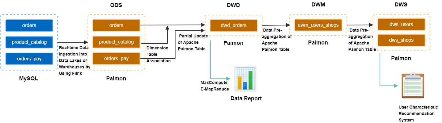
Build the ODS layer: Real-time ingestion of business database data into the data warehouse.
A MySQL database has three business tables: an orders table, an orders_pay table, and a product_catalog dictionary table. Flink writes data from these tables to OSS in real time. The data is stored in the Paimon format as the ODS layer.Build the DWD layer: Create a topic-based wide table.
The orders table, product_catalog table, and orders_pay table are widened using Paimon's partial-update merge mechanism. This generates a DWD layer wide table and produces a changelog with minute-level latency.Build the DWS layer: Calculate metrics.
Flink consumes the changelog of the wide table in real time. It uses Paimon's pre-aggregation merge mechanism to produce the DWM layer `dwm_users_shops` (user-merchant aggregate intermediate table). It finally produces the DWS layer `dws_users` (user aggregate metric table) and `dws_shops` (merchant aggregate metric table).
Prerequisites
You have activated Data Lake Formation. We recommend that you use DLF 2.5 as the storage service. For more information, see Get started with DLF.
You have activated fully managed Flink. For more information, see Activate Realtime Compute for Apache Flink.
You have activated StarRocks in EMR. For more information, see Quickly use a compute-storage separated instance.
The StarRocks instance, DLF, and Flink workspace must be in the same region.
Limits
Only Ververica Runtime (VVR) 11.1.0 and later support this streaming data lakehouse solution.
Build a streaming data lakehouse
Prepare a MySQL CDC data source
This topic uses an ApsaraDB RDS for MySQL instance as an example. You need to create a database named order_dw and populate three business tables with data.
Create an ApsaraDB RDS for MySQL instance.
ImportantThe ApsaraDB RDS for MySQL instance must be in the same VPC as the Flink workspace. If they are not in the same VPC, see How do I access other services across VPCs?
Create a database and an account (Deprecated, redirects to "Step 1").
Create a database named order_dw. Create a privileged account or a standard account with read and write permissions on the order_dw database.
Create three tables and insert data into them.
CREATE TABLE `orders` (
  order_id bigint not null primary key,
  user_id varchar(50) not null,
  shop_id bigint not null,
  product_id bigint not null,
  buy_fee bigint not null,
  create_time timestamp not null,
  update_time timestamp not null default now(),
  state int not null
);

CREATE TABLE `orders_pay` (
  pay_id bigint not null primary key,
  order_id bigint not null,
  pay_platform int not null,
  create_time timestamp not null
);

CREATE TABLE `product_catalog` (
  product_id bigint not null primary key,
  catalog_name varchar(50) not null
);

-- Prepare data.
INSERT INTO product_catalog VALUES(1, 'phone_aaa'),(2, 'phone_bbb'),(3, 'phone_ccc'),(4, 'phone_ddd'),(5, 'phone_eee');

INSERT INTO orders VALUES
(100001, 'user_001', 12345, 1, 5000, '2023-02-15 16:40:56', '2023-02-15 18:42:56', 1),
(100002, 'user_002', 12346, 2, 4000, '2023-02-15 15:40:56', '2023-02-15 18:42:56', 1),
(100003, 'user_003', 12347, 3, 3000, '2023-02-15 14:40:56', '2023-02-15 18:42:56', 1),
(100004, 'user_001', 12347, 4, 2000, '2023-02-15 13:40:56', '2023-02-15 18:42:56', 1),
(100005, 'user_002', 12348, 5, 1000, '2023-02-15 12:40:56', '2023-02-15 18:42:56', 1),
(100006, 'user_001', 12348, 1, 1000, '2023-02-15 11:40:56', '2023-02-15 18:42:56', 1),
(100007, 'user_003', 12347, 4, 2000, '2023-02-15 10:40:56', '2023-02-15 18:42:56', 1);

INSERT INTO orders_pay VALUES
(2001, 100001, 1, '2023-02-15 17:40:56'),
(2002, 100002, 1, '2023-02-15 17:40:56'),
(2003, 100003, 0, '2023-02-15 17:40:56'),
(2004, 100004, 0, '2023-02-15 17:40:56'),
(2005, 100005, 0, '2023-02-15 18:40:56'),
(2006, 100006, 0, '2023-02-15 18:40:56'),
(2007, 100007, 0, '2023-02-15 18:40:56');
Manage metadata
Create a Paimon Catalog
Log on to the Realtime Compute for Apache Flink console.
In the navigation pane on the left, go to the Metadata Management page and click Create Catalog.
On the Built-in Catalog tab, click Apache Paimon, and then click Next.
Enter the following parameters, select DLF as the storage type, and click OK.
Configuration item
Description
Required
Remarks
metastore
The metastore type.
Yes
In this example, select dlf.
catalog name
The name of the DLF data catalog.
ImportantIf you use a Resource Access Management (RAM) user or role, make sure you have read and write permissions on the DLF data. For more information, see Data authorization management.
Yes
We recommend using DLF 2.5. You do not need to enter an AccessKey or other information. You can quickly select an existing DLF data catalog. To create a data catalog, see Data catalog.
After you create a data catalog named paimoncatalog, select it from the list.
Create the order_dw database in the data catalog. This database is used to synchronize data from all tables in the order_dw database in MySQL.
In the navigation pane on the left, choose . Click New to create a temporary query.
-- Use the paimoncatalog data source.
USE CATALOG paimoncatalog;
-- Create the order_dw database.
CREATE DATABASE order_dw;
A
The following statement has been executed successfully!message indicates that the database was created.
For more information about how to use a Paimon Catalog, see Manage Paimon Catalogs.
Create a MySQL Catalog
On the Metadata Management page, click Create Catalog.
On the Built-in Catalog tab, click MySQL, and then click Next.
Enter the following parameters and click OK to create a MySQL catalog named mysqlcatalog.
Configuration item
Description
Required
Remarks
catalog name
The name of the catalog.
Yes
Enter a custom name in English. This topic uses mysqlcatalog as an example.
hostname
The IP address or hostname of the MySQL database.
Yes
For more information, see View and manage instance endpoints and ports. Because the ApsaraDB RDS for MySQL instance and the fully managed Flink workspace are in the same VPC, enter the private network address.
port
The port number of the MySQL database service. The default value is 3306.
No
For more information, see View and manage instance endpoints and ports.
default-database
The name of the default MySQL database.
Yes
Enter the name of the database to synchronize, which is order_dw in this topic.
username
The username for the MySQL database service.
Yes
This is the account created in the Prepare a MySQL CDC data source section.
password
The password for the MySQL database service.
Yes
This is the password for the account created in the Prepare a MySQL CDC data source section.
Build the ODS layer: Real-time ingestion of business database data
Use Flink Change Data Capture (CDC) and a YAML data ingestion job to synchronize data from MySQL to Paimon. This builds the ODS layer in a single step.
Create and start the YAML data ingestion job.
In the Realtime Compute for Apache Flink console, on the page, create a blank YAML draft job named ods.
Copy the following code into the editor. Make sure to modify parameters such as the username and password.
source:
  type: mysql
  name: MySQL Source
  hostname: rm-bp1e********566g.mysql.rds.aliyuncs.com
  port: 3306
  username: ${secret_values.username}
  password: ${secret_values.password}
  tables: order_dw.\.*  # Use a regular expression to read all tables in the order_dw database.
  # (Optional) Synchronize data from tables newly created during the incremental phase.
  scan.binlog.newly-added-table.enabled: true
  # (Optional) Synchronize table and field comments.
  include-comments.enabled: true
  # (Optional) Prioritize dispatching unbounded chunks to prevent potential TaskManager OutOfMemory errors.
  scan.incremental.snapshot.unbounded-chunk-first.enabled: true
  # (Optional) Enable parsing filters to accelerate reads.
  scan.only.deserialize.captured.tables.changelog.enabled: true

sink:
  type: paimon
  name: Paimon Sink
  catalog.properties.metastore: rest
  catalog.properties.uri: http://cn-beijing-vpc.dlf.aliyuncs.com
  catalog.properties.warehouse: paimoncatalog
  catalog.properties.token.provider: dlf

pipeline:
  name: MySQL to Paimon Pipeline
Configuration item
Description
Required
Example
catalog.properties.metastoreThe metastore type. The value is fixed to rest.
Yes
rest
catalog.properties.token.providerThe token provider. The value is fixed to dlf.
Yes
dlf
catalog.properties.uriThe URI to access the DLF Rest Catalog Server. The format is
http://[region-id]-vpc.dlf.aliyuncs.com. For more information about Region IDs, see Endpoints.Yes
http://cn-beijing-vpc.dlf.aliyuncs.com
catalog.properties.warehouseThe name of the DLF Catalog.
Yes
paimoncatalog
For more information about how to optimize Paimon write performance, see Paimon performance optimization.
In the upper-right corner, click Deploy.
On the page, find the ods job that you just deployed. In the Actions column, click Start. Select Stateless Start to start the job. For more information about job start configurations, see Start a job.
View the data of the three tables synchronized from MySQL to Paimon.
On the Query Script tab of the page in the Realtime Compute for Apache Flink console, copy the following code into the query script. Select the code snippet and click Run in the upper-right corner.
SELECT * FROM paimoncatalog.order_dw.orders ORDER BY order_id;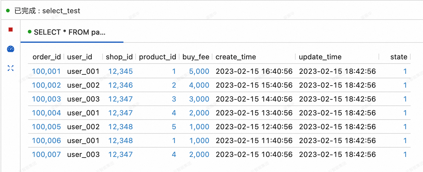
Build the DWD layer: A topic-based wide table
Create the DWD layer Paimon wide table dwd_orders
On the Query Script tab of the page in the Realtime Compute for Apache Flink console, copy the following code into the query script. Select the code snippet and click Run in the upper-right corner.
CREATE TABLE paimoncatalog.order_dw.dwd_orders (
    order_id BIGINT,
    order_user_id STRING,
    order_shop_id BIGINT,
    order_product_id BIGINT,
    order_product_catalog_name STRING,
    order_fee BIGINT,
    order_create_time TIMESTAMP,
    order_update_time TIMESTAMP,
    order_state INT,
    pay_id BIGINT,
    pay_platform INT COMMENT 'platform 0: phone, 1: pc',
    pay_create_time TIMESTAMP,
    PRIMARY KEY (order_id) NOT ENFORCED
) WITH (
    'merge-engine' = 'partial-update', -- Use the partial-update merge engine to generate the wide table.
    'changelog-producer' = 'lookup' -- Use the lookup changelog producer to generate changelogs with low latency.
);
A
Query has been executedmessage indicates that the table was created.Consume changelogs from the ODS layer tables orders and orders_pay in real time
In the Realtime Compute for Apache Flink console, on the page, create an SQL stream job named dwd, copy the following code into the SQL editor, Deploy the job, and then Start it statelessly.
This SQL job performs a dimension table join between the orders table and the product_catalog table. The result of the join, along with data from the orders_pay table, is written to the dwd_orders table. The partial-update merge engine of Paimon is used to widen the data for records with the same order_id in the orders and orders_pay tables.
SET 'execution.checkpointing.max-concurrent-checkpoints' = '3';
SET 'table.exec.sink.upsert-materialize' = 'NONE';

SET 'execution.checkpointing.interval' = '10s';
SET 'execution.checkpointing.min-pause' = '10s';

-- Paimon does not currently support multiple INSERT statements into the same table within a single job. Therefore, use UNION ALL.
INSERT INTO paimoncatalog.order_dw.dwd_orders
SELECT
    o.order_id,
    o.user_id,
    o.shop_id,
    o.product_id,
    dim.catalog_name,
    o.buy_fee,
    o.create_time,
    o.update_time,
    o.state,
    NULL,
    NULL,
    NULL
FROM
    paimoncatalog.order_dw.orders o
    LEFT JOIN paimoncatalog.order_dw.product_catalog FOR SYSTEM_TIME AS OF proctime() AS dim
    ON o.product_id = dim.product_id
UNION ALL
SELECT
    order_id,
    NULL,
    NULL,
    NULL,
    NULL,
    NULL,
    NULL,
    NULL,
    NULL,
    pay_id,
    pay_platform,
    create_time
FROM
    paimoncatalog.order_dw.orders_pay;
View data in the dwd_orders wide table
On the Query Script tab of the page in the Realtime Compute for Apache Flink console, copy the following code into the query script. Select the code snippet and click Run in the upper-right corner.
SELECT * FROM paimoncatalog.order_dw.dwd_orders ORDER BY order_id;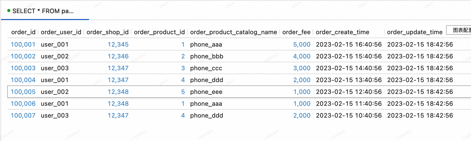
Build the DWS layer: Metric calculation
Create the DWS layer aggregation tables dws_users and dws_shops
On the Query Script tab of the page in the Realtime Compute for Apache Flink console, copy the following code into the query script. Select the code snippet and click Run in the upper-right corner.
-- User-dimension aggregate metric table.
CREATE TABLE paimoncatalog.order_dw.dws_users (
    user_id STRING,
    ds STRING,
    paid_buy_fee_sum BIGINT COMMENT 'Total amount paid on the current day',
    PRIMARY KEY (user_id, ds) NOT ENFORCED
) WITH (
    'merge-engine' = 'aggregation', -- Use the aggregation merge engine to generate the aggregation table.
    'fields.paid_buy_fee_sum.aggregate-function' = 'sum' -- Sum the data in the paid_buy_fee_sum field to produce the aggregate result.
    -- Because the dws_users table is not consumed downstream in a streaming fashion, you do not need to specify a changelog producer.
);

-- Merchant-dimension aggregate metric table.
CREATE TABLE paimoncatalog.order_dw.dws_shops (
    shop_id BIGINT,
    ds STRING,
    paid_buy_fee_sum BIGINT COMMENT 'Total amount paid on the current day',
    uv BIGINT COMMENT 'Total number of unique purchasing users on the current day',
    pv BIGINT COMMENT 'Total number of purchases by users on the current day',
    PRIMARY KEY (shop_id, ds) NOT ENFORCED
) WITH (
    'merge-engine' = 'aggregation', -- Use the aggregation merge engine to generate the aggregation table.
    'fields.paid_buy_fee_sum.aggregate-function' = 'sum', -- Sum the data in the paid_buy_fee_sum field to produce the aggregate result.
    'fields.uv.aggregate-function' = 'sum', -- Sum the data in the uv field to produce the aggregate result.
    'fields.pv.aggregate-function' = 'sum' -- Sum the data in the pv field to produce the aggregate result.
    -- Because the dws_shops table is not consumed downstream in a streaming fashion, you do not need to specify a changelog producer.
);

-- To calculate aggregation tables from both the user and merchant perspectives simultaneously, create an intermediate table with a composite primary key of user and merchant.
CREATE TABLE paimoncatalog.order_dw.dwm_users_shops (
    user_id STRING,
    shop_id BIGINT,
    ds STRING,
    paid_buy_fee_sum BIGINT COMMENT 'Total amount paid by the user at the merchant on the current day',
    pv BIGINT COMMENT 'Number of times the user purchased at the merchant on the current day',
    PRIMARY KEY (user_id, shop_id, ds) NOT ENFORCED
) WITH (
    'merge-engine' = 'aggregation', -- Use the aggregation merge engine to generate the aggregation table.
    'fields.paid_buy_fee_sum.aggregate-function' = 'sum', -- Sum the data in the paid_buy_fee_sum field to produce the aggregate result.
    'fields.pv.aggregate-function' = 'sum', -- Sum the data in the pv field to produce the aggregate result.
    'changelog-producer' = 'lookup', -- Use the lookup changelog producer to generate changelogs with low latency.
    -- The intermediate table at the DWM layer is generally not queried directly by upper-layer applications, so you can optimize its write performance.
    'file.format' = 'avro', -- The Avro row store format provides more efficient write performance.
    'metadata.stats-mode' = 'none' -- Discarding statistics increases the cost of online analytical processing (OLAP) queries but improves write performance. This does not affect continuous stream processing.
);
A response of
Query has been executedindicates that the creation was successful.Change data in the dwd_orders table in the DWD layer
On the tab of the Realtime Compute for Apache Flink console, create a new SQL stream job named dwm. Copy the following code into the SQL editor, deploy the job, and then start it statelessly.
This SQL job writes data from the dwd_orders table to the dwm_users_shops table. It uses the pre-aggregation merge engine of Paimon to automatically sum the order_fee to calculate the total consumption amount per user per merchant. It also sums the value 1 to calculate the number of purchases per user per merchant.
SET 'execution.checkpointing.max-concurrent-checkpoints' = '3';
SET 'table.exec.sink.upsert-materialize' = 'NONE';

SET 'execution.checkpointing.interval' = '10s';
SET 'execution.checkpointing.min-pause' = '10s';

INSERT INTO paimoncatalog.order_dw.dwm_users_shops
SELECT
    order_user_id,
    order_shop_id,
    DATE_FORMAT (pay_create_time, 'yyyyMMdd') as ds,
    order_fee,
    1 -- One input record represents one purchase.
FROM paimoncatalog.order_dw.dwd_orders
WHERE pay_id IS NOT NULL AND order_fee IS NOT NULL;
Consume changelogs from the DWM layer table dwm_users_shops in real time
On the page of the Realtime Compute for Apache Flink console, create a new SQL stream job named dws. Copy the following code into the SQL editor, deploy the job, and then start it statelessly.
This SQL job writes data from the dwm_users_shops table to the dws_users and dws_shops tables. It uses the pre-aggregation merge engine of Paimon to calculate the total consumption amount for each user (paid_buy_fee_sum) in the dws_users table. In the dws_shops table, it calculates the total revenue for each merchant (paid_buy_fee_sum), the number of purchasing users (by summing 1), and the total number of purchases (pv).
SET 'execution.checkpointing.max-concurrent-checkpoints' = '3';
SET 'table.exec.sink.upsert-materialize' = 'NONE';

SET 'execution.checkpointing.interval' = '10s';
SET 'execution.checkpointing.min-pause' = '10s';

-- Unlike the DWD job, each INSERT statement here writes to a different Paimon table, so they can be in the same job.
BEGIN STATEMENT SET;

INSERT INTO paimoncatalog.order_dw.dws_users
SELECT
    user_id,
    ds,
    paid_buy_fee_sum
FROM paimoncatalog.order_dw.dwm_users_shops;

-- The primary key is the merchant. The data volume for some popular merchants may be much higher than for others.
-- Therefore, use local merge to pre-aggregate data in memory before writing to Paimon. This helps mitigate data skew.
INSERT INTO paimoncatalog.order_dw.dws_shops /*+ OPTIONS('local-merge-buffer-size' = '64mb') */
SELECT
    shop_id,
    ds,
    paid_buy_fee_sum,
    1, -- One input record represents all consumption by one user at that merchant.
    pv
FROM paimoncatalog.order_dw.dwm_users_shops;

END;
View data in the dws_users and dws_shops tables
On the Query Script tab of the page in the Realtime Compute for Apache Flink console, copy the following code into the query script. Select the code snippet and click Run in the upper-right corner.
--View data in the dws_users table.
SELECT * FROM paimoncatalog.order_dw.dws_users ORDER BY user_id;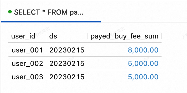
--View data in the dws_shops table.
SELECT * FROM paimoncatalog.order_dw.dws_shops ORDER BY shop_id;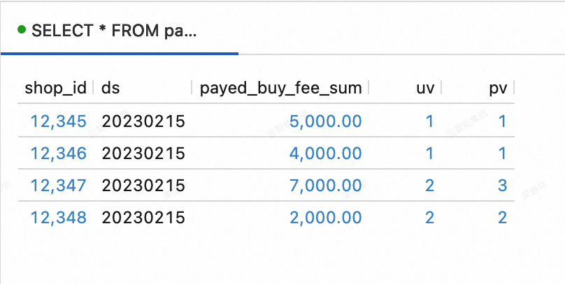
Capture changes in the business database
After the streaming data lakehouse is built, you can test its ability to capture changes from the business database.
Insert the following data into the order_dw database in MySQL.
INSERT INTO orders VALUES
(100008, 'user_001', 12345, 3, 3000, '2023-02-15 17:40:56', '2023-02-15 18:42:56', 1),
(100009, 'user_002', 12348, 4, 1000, '2023-02-15 18:40:56', '2023-02-15 19:42:56', 1),
(100010, 'user_003', 12348, 2, 2000, '2023-02-15 19:40:56', '2023-02-15 20:42:56', 1);

INSERT INTO orders_pay VALUES
(2008, 100008, 1, '2023-02-15 18:40:56'),
(2009, 100009, 1, '2023-02-15 19:40:56'),
(2010, 100010, 0, '2023-02-15 20:40:56');
View data in the dws_users and dws_shops tables. On the Query Script tab of the page in the Realtime Compute for Apache Flink console, copy the following code into the query script. Select the code snippet and click Run in the upper-right corner.
dws_users table
SELECT * FROM paimoncatalog.order_dw.dws_users ORDER BY user_id;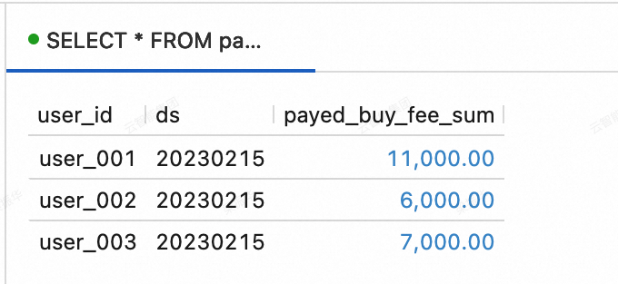
dws_shops table
SELECT * FROM paimoncatalog.order_dw.dws_shops ORDER BY shop_id;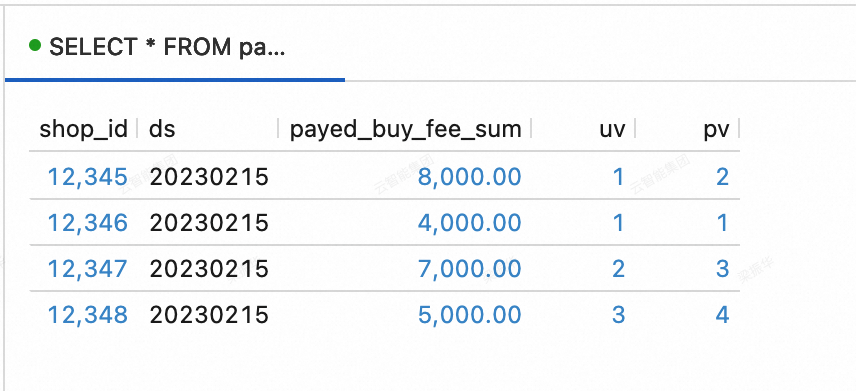
Use the streaming data lakehouse
The previous section showed how to create a Paimon Catalog and write to Paimon tables in Flink. This section shows some simple scenarios for data analytics using StarRocks after you build the streaming data lakehouse.
First, log on to the StarRocks instance and create a catalog for oss-paimon. For more information, see Paimon Catalog.
CREATE EXTERNAL CATALOG paimon_catalog
PROPERTIES
(
    'type' = 'paimon',
    'paimon.catalog.type' = 'filesystem',
    'aliyun.oss.endpoint' = 'oss-cn-beijing-internal.aliyuncs.com',
    'paimon.catalog.warehouse' = 'oss://<bucket>/<object>'
);
Property | Required | Remarks |
type | Yes | The data source type. The value is paimon. |
paimon.catalog.type | Yes | The metastore type used by Paimon. This example uses filesystem as the metastore type. |
aliyun.oss.endpoint | Yes | If you use OSS or OSS-HDFS as the warehouse, you must specify the corresponding endpoint. |
paimon.catalog.warehouse | Yes | The format is oss://<bucket>/<object>. In this format:
You can view your bucket and object names in the OSS console. |
Ranking query
Analyze the DWS layer aggregation table. The following example shows how to use StarRocks to query the top three merchants with the highest transaction amounts on February 15, 2023.
SELECT ROW_NUMBER() OVER (ORDER BY paid_buy_fee_sum DESC) AS rn, shop_id, paid_buy_fee_sum
FROM dws_shops
WHERE ds = '20230215'
ORDER BY rn LIMIT 3;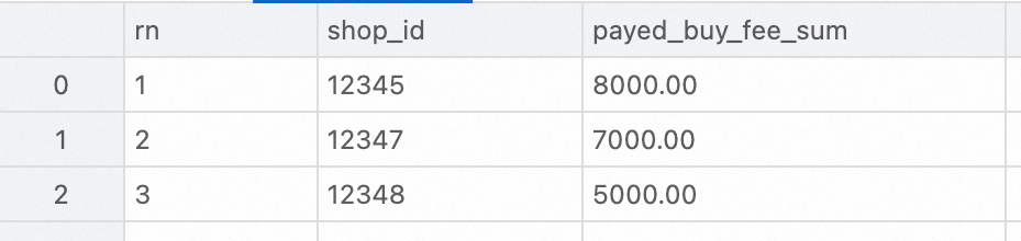
Details query
This example shows how to analyze the DWD layer wide table using StarRocks to query the order details for a specific customer who paid using a specific payment platform in February 2023.
SELECT * FROM dwd_orders
WHERE order_create_time >= '2023-02-01 00:00:00' AND order_create_time < '2023-03-01 00:00:00'
AND order_user_id = 'user_001'
AND pay_platform = 0
ORDER BY order_create_time;;
Data report
The following example shows how to analyze the DWD layer wide table. You can use StarRocks to query the total number of orders and the total order amount for each product category in February 2023.
SELECT
  order_create_time AS order_create_date,
  order_product_catalog_name,
  COUNT(*),
  SUM(order_fee)
FROM
  dwd_orders
WHERE
  order_create_time >= '2023-02-01 00:00:00'  and order_create_time < '2023-03-01 00:00:00'
GROUP BY
  order_create_date, order_product_catalog_name
ORDER BY
  order_create_date, order_product_catalog_name;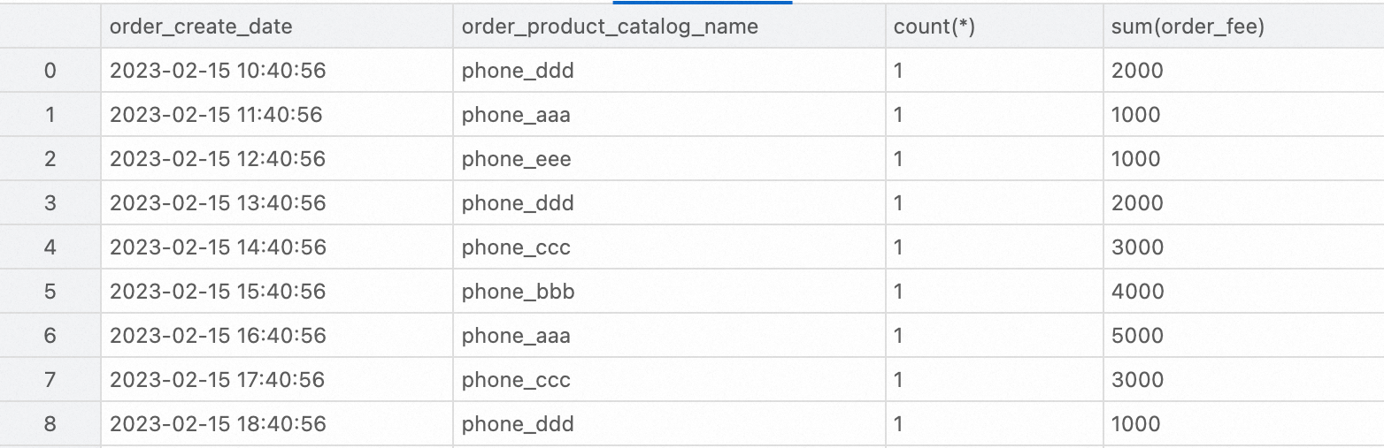
References
To build an offline Paimon data lakehouse using Flink's batch processing capabilities, see Quick start for Flink batch processing.