AnalyticDB:Build an end-to-end machine learning pipeline using AnalyticDB for MySQL and DMS

Overall architecture

To address these challenges, we built an integrated solution based on AnalyticDB for MySQL and DMS. The overall architecture is shown in the following diagram:

Core component breakdown

• AnalyticDB for MySQL: Compute and storage engine
  As the compute and storage core of this solution, it provides a built-in distributed Spark engine and unified data lake management. It performs large-scale feature engineering computations and stores intermediate data efficiently in Delta Lake or Apache Iceberg format, enabling visual data asset management and high-performance queries.
  
  

• Data Management (DMS): Development and orchestration hub
  As the development and orchestration hub, it offers fully managed Notebook, Airflow, and MLflow services to seamlessly connect the entire MLOps loop:
  
  

  • Notebook: Provides data scientists with an interactive environment for data exploration, model training, and algorithm validation.

  • Airflow: Converts validated data and model pipelines into stable, reliable production tasks with periodic scheduling.

• Delta Lake on AnalyticDB for MySQL: Unified data lake foundation
  As the unified data lake foundation, its key value lies in ACID transaction guarantees. This ensures that during high-concurrency writes of factor data, downstream backtesting or training jobs never read partially written dirty data, guaranteeing accuracy and reproducibility of business results.
  
  

AnalyticDB for MySQL setup

Ensure you have created an AnalyticDB for MySQL instance and completed the following configurations:

1. Create a database account: Create a database account with appropriate permissions based on your access method.

   • If you access the instance using an Alibaba Cloud account, create a privileged account.

   • If you access the instance using a Resource Access Management (RAM) user, create a privileged account, grant a standard account the necessary database and table permissions, and bind the RAM user to the standard account.

2. Create a Job-type resource group: In the Cluster Management > Resource Management > Resource Groups section, create a dedicated compute resource group for Spark jobs. For more information, see Interactive resource group properties.

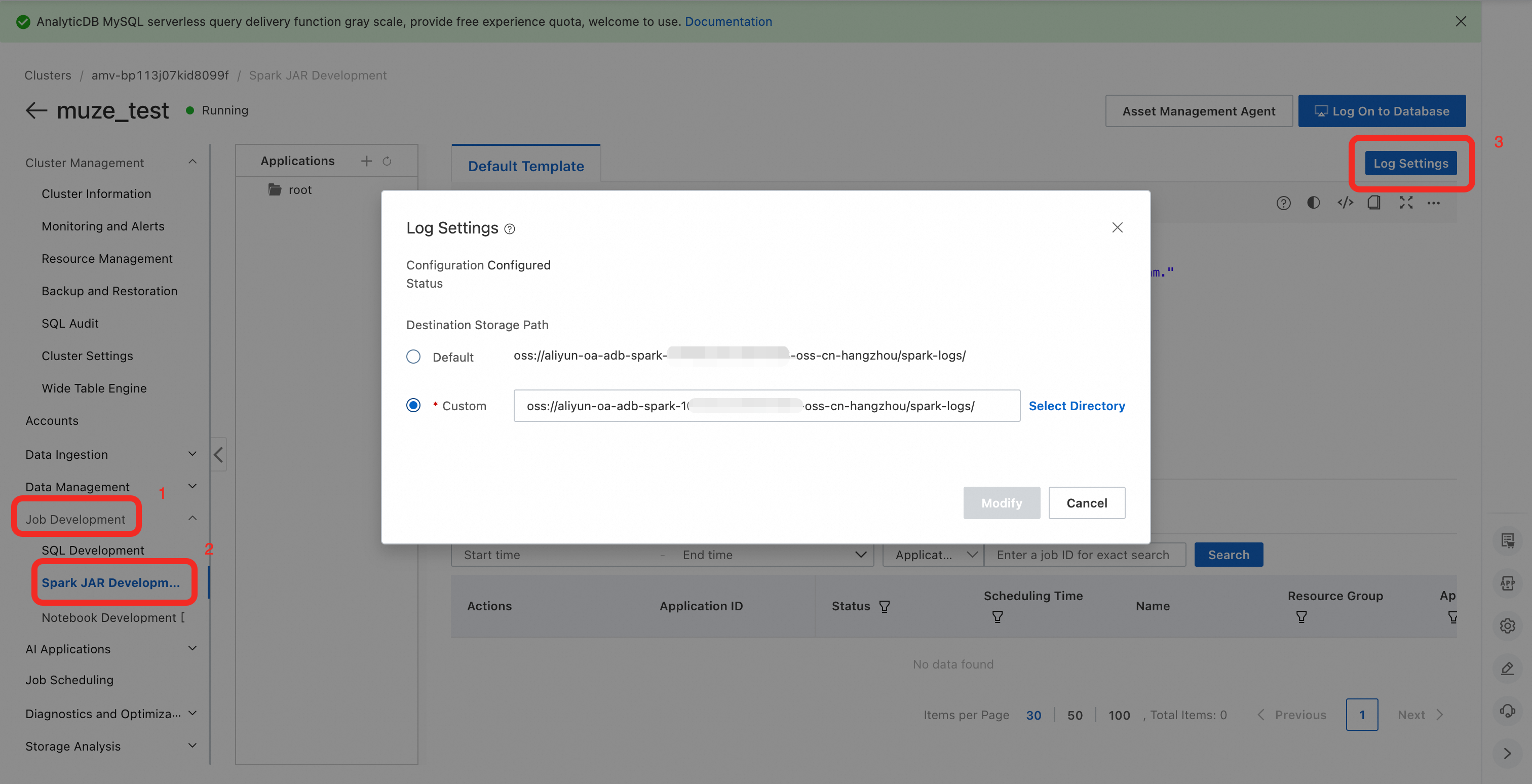
3. Configure Spark log storage: Set an OSS path in the console to store logs for Spark applications.

   1. Log on to the AnalyticDB for MySQL console and select the region of your cluster in the upper-left corner.

   2. In the navigation pane on the left, click Clusters and then click the target cluster ID.

   3. In the navigation pane on the left, choose Job Development > Spark JAR Development.

   4. Click Log Settings and select either the Default path or a Custom storage path.

      Note

      When using a custom path, do not save logs in the root directory of your OSS bucket. Ensure the path includes at least one subfolder.

      

4. Grant permissions to RAM users (optional): If you use a RAM user for development, ensure it has been granted permissions to access Spark and OSS.

5. Upload dependency JAR packages: Download the MLflow-related Spark JAR package and upload it to your OSS bucket in advance.

DMS Notebook setup

1. Access DMS Notebook:

   • Log on to the AnalyticDB for MySQL console and select the region of your cluster in the upper-left corner.

   • In the navigation pane on the left, click Clusters and then click the target cluster ID.

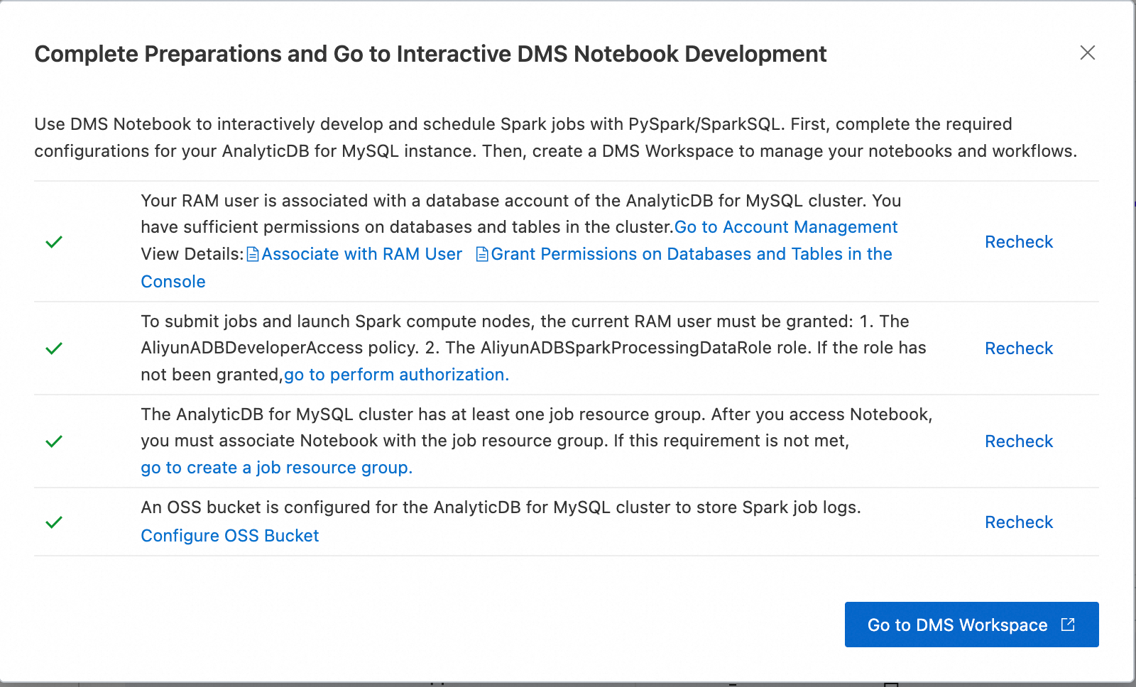
   • In the navigation pane on the left under cluster management, choose Job Development > Notebook Development.

• After completing the prerequisites, click Go to DMS Workspace.

  

• Create a workspace and data source:

  • In the Create workspace dialog box, enter a workspace name.

  • In the Add managed instance or import project dialog box, enter the privileged account and password for your AnalyticDB for MySQL instance.

    Note

    On first connection, network issues may cause failures. In the warning dialog, click Set whitelist. The system will automatically add DMS IP ranges to your instance whitelist to ensure connectivity.

• Create and configure a Spark cluster: On the DMS resource management page, create a new Spark cluster.

  Note

  This does not create a new physical Spark cluster. Instead, it establishes a binding relationship that defines which AnalyticDB for MySQL instance’s Job resource group receives Spark jobs, along with the default resource usage range (Executor_size × min_count to Executor_size × max_count).

  • Click the button to go to the Resource management page.

  • Click Compute clusters and select the Spark clusters tab.

  • Click Create cluster and configure the following parameters:

    Parameter	Description	Example
    Cluster type	Type of compute cluster	Spark cluster
    Cluster name	Enter a descriptive name for your use case.	spark_test
    Runtime image	Select from the following images: adb-spark:v3.3-scala2.12-python3.9 adb-spark:v3.5-scala2.12-python3.11	adb-spark:v3.5-scala2.12-python3.11 Note To run the example in the Appendix, ensure runtime consistency.
    AnalyticDB instance	Select your AnalyticDB for MySQL cluster from the drop-down list.	amv-uf6i4bi88****
    AnalyticDB MySQL resource group	Select a Job-type resource group from the drop-down list.	testjob
    Spark APP Executor specification	Select the resource specification for Spark Executors. Different model values correspond to different specs. For details, see the model column in Spark application configuration parameters.	large
    vSwitch	Select a vSwitch in your current VPC.	vsw-uf6n9ipl6qgo****
    Metadata	Metadata source	Engine metadata
    Dependency JARs	OSS path of the JAR file. Enter the OSS path of the downloaded JAR. If you specify the JAR path directly in your code, leave this blank.	oss://testBucketName/jar_file/mssql-jdbc-12.8.1.jre8.jar

  • Click OK to complete cluster creation.

• Create and start a Notebook session

  Note

  The Notebook session provides a single-machine Python environment for data science development and lets you manage Python dependencies in bulk. The first startup takes about 5 minutes. Be patient.

  • Click the button to go to the Resource management page.

  • Click Notebook sessions.

  • Click Create session and configure the following parameters:

    Parameter	Description	Example
    Session name	You can customize the session name.	new_session
    Associated cluster	Select the Spark cluster created in the previous step.	spark_test
    Image	Select the image specification.	Spark3.5_Scala2.12_Python3.11:1.0.9 Note To run the example in the Appendix, ensure runtime consistency.
    Specification	Kernel resource specification. For machine learning scenarios, use at least 8 cores.	4C16G
    Configuration	Profile resources. You can edit the profile name, auto-release duration, data storage location, PyPI package management, and environment variables. Auto-release duration: If idle longer than this duration, resources are automatically released. Setting it to 0 means resources are never auto-released.	default_profile
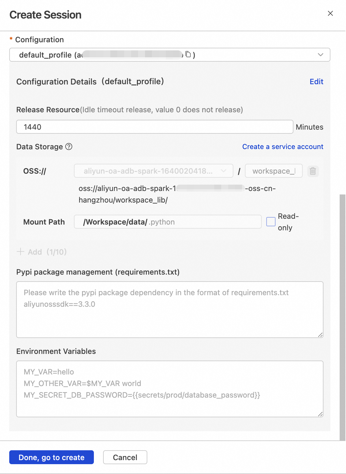
    Profile details > Data storage > OSS	Select a bucket in the same region and define a subpath. In Spark ML scenarios, this OSS path distributes Python dependencies between the Notebook kernel and Spark worker nodes.	oss://your-bucket/spark-deps/
    Configuration Details > Data Storage > Mount Path	Set to .python	.python

    Important

    The session profile must be configured with OSS access permissions:

    • Select a bucket in the same region. Use a new, empty subpath.

    • Set the mount path to .python.

    • Authorize after saving.

  • After saving, return to the Notebook sessions list and click Start to launch the session.

• Create a Notebook file

  • Click the button.

  • In the CODE module, right-click and select New Notebook file.

DMS MLflow setup

For detailed MLflow configuration instructions, see DMS MLflow User Guide. After creation, manually add the IPv4 CIDR block of the VPC where your Notebook resides to the access control list (ACL) of the MLflow Application Load Balancer (ALB).

Step 1: Install Python dependencies and distribute them to the distributed environment

In the Notebook, run the following commands to install dependencies in the single-machine Python environment and use the pyp_persist command to distribute Python packages to Spark executor nodes, ensuring consistency across the distributed environment.

1. Update system packages and install build tools:

   !apt update && apt -y install build-essential

2. Uninstall default Python packages:

   !pip uninstall -y scikit-learn pandas xgboost scipy PyArrow joblib threadpoolctl numpy python-dateutil six pytz

3. Install required Python packages:

   !pip install xgboost scikit-learn pandas==2.0.2 PyArrow scipy joblib threadpoolctl python-dateutil six numpy==1.26.4

4. Persist the Python environment to Spark nodes:

   !pyp_persist

Step 2: Start the Spark application and validate the environment

1. Start a Spark Session:

   from pyspark.sql import SparkSession
   
   spark = SparkSession.builder.appName("MachineLearning") \
       .config("spark.dynamicAllocation.enabled", "false") \
       .config("spark.executor.instances", "4") \
       .config("spark.jars", f"oss://<your_bucket>/mlflow-spark_2.12-3.5.1.jar")\
       .getOrCreate()

2. Verify that Python packages are correctly distributed to Spark nodes:

   import socket
   
   def check_pandas_on_executor(x):
       try:
           import pandas as pd
           return (socket.gethostname(), f"pandas:{pd.__version__}")
       except ImportError as e:
           return (socket.gethostname(), "FAILED", str(e))
   
   nodes_info = spark.sparkContext.parallelize(range(10), 10) \
                     .map(check_pandas_on_executor) \
                     .distinct() \
                     .collect()
   
   print("Executor python env check: ")
   for info in nodes_info:
       print(info)

Step 3: Generate a trading dataset

The following code generates simulated stock trading data to demonstrate a complete machine learning workflow.

1. Define the OSS storage path:

   OSS_BUCKET = "<your_data_bucket>"
   OSS_ROOT_PATH = f"oss://{OSS_BUCKET}/demo20260302_tmp/"

2. Generate mock data and write to OSS:

   import os
   import pandas as pd
   import numpy as np
   from pyspark.sql import SparkSession
   from pyspark.sql.types import *
   
   OSS_OUTPUT_PATH = f"{OSS_ROOT_PATH}raw_market_data"
   
   print(">>> Start generating mock market data...")
   
   def generate_mock_data():
       start_date = "20230101"
       end_date = "20231231"
       date_range = pd.date_range(start=start_date, end=end_date, freq='D')
       num_stocks = 20  # Base number of shares
       
       # --- Generate basic stock data ---
       dfs = []
       for i in range(num_stocks):
           symbol = f"MOCK_{i:04d}"  # Generate virtual stock codes
           
           # Generate price series (simulating reasonable volatility)
           base_price = np.random.uniform(10, 100)  # The base price is between 10 and 100.
           price_series = [base_price]
           for _ in range(1, len(date_range)):
               # Daily price fluctuations: Random fluctuations within ±5%
               change = np.random.normal(0, 0.02)
               price_series.append(max(1, price_series[-1] * (1 + change)))
           
           # Generate trading volume (related to price).
           volume_series = [np.random.poisson(price * 1000) for price in price_series]
           
           # Create a DataFrame
           df = pd.DataFrame({
               "date": date_range,
               "ticker": symbol,
               "open": price_series,
               "high": [p * np.random.uniform(1, 1.02) for p in price_series],
               "low": [p * np.random.uniform(0.98, 1) for p in price_series],
               "close": price_series,
               "volume": volume_series})
           
           # Ensure the type is correct
           df['date'] = df['date'].astype(str)
           df['volume'] = df['volume'].astype(float)
           
           dfs.append(df)
       
       full_df = pd.concat(dfs)
       
       # --- Data Augmentation: Simulating Large Data Volumes ---
       print(">>> Perform data fission to simulate massive amounts of data...")
       aug_dfs = []
       # Split 20 stocks into 1000 virtual stocks
       for i in range(50): 
           temp = full_df.copy()
           # Modify the ticker name, for example, MOCK_0000_001
           temp['ticker'] = temp['ticker'] + f"_{i:03d}"
           # Add small random perturbations to simulate different trends.
           noise = np.random.normal(1, 0.005, len(temp))
           for col in ['open', 'high', 'low', 'close']:
               temp[col] = temp[col] * noise
           aug_dfs.append(temp)
           
       return pd.concat(aug_dfs)
   
   # Generate mock data
   pdf = generate_mock_data()
   print(f">>> Data is ready; Pandas DataFrame structure:{pdf.shape}")
   print(">>> Converting to Spark DataFrame...")
   
   # Defining a schema is more robust and avoids errors in automatic inference.
   schema = StructType([
       StructField("date", StringType(), True),
       StructField("ticker", StringType(), True),
       StructField("open", DoubleType(), True),
       StructField("high", DoubleType(), True),
       StructField("low", DoubleType(), True),
       StructField("close", DoubleType(), True),
       StructField("volume", DoubleType(), True)
   ])
   
   # Create DataFrame (Optimize transmission using Arrow)
   sdf = spark.createDataFrame(pdf, schema=schema)
   
   print(f">>> Writing to OSS:{OSS_OUTPUT_PATH} ...")
   
   # Write to Parquet files
   # mode("overwrite"): Overwrite mode, suitable for repeated runs of the demo
   # partitionBy("date"): Partition by date, crucial for subsequent Delta Lake or Hive queries
   (sdf.write
       .mode("overwrite")
       .partitionBy("date")
       .parquet(OSS_OUTPUT_PATH))
   
   print(">>> Writing complete!")

Step 4: Create a Delta Lake table and write data

Delta Lake provides ACID transaction support to ensure data consistency.

1. Create a database:

   DATABASE_LOCATION = f"{OSS_ROOT_PATH}db_location/"
   DB_NAME = 'stockdata'

   spark.sql(f"DROP DATABASE IF EXISTS {DB_NAME};")
   spark.sql(f"CREATE DATABASE IF NOT EXISTS {DB_NAME} LOCATION '{DATABASE_LOCATION}';")

2. Create a Delta Lake table and append day-level partitioned Parquet files from OSS to the table DB_MARKET.bronze_market_data.

   # Read the data (make sure it includes a date column).
   path = OSS_OUTPUT_PATH + "/date=2023-01-03/"
   raw_df = spark.read \
       .option("basePath", OSS_OUTPUT_PATH) \
       .parquet(path)
   (raw_df.write.format("delta")
       .mode("append")              
       .option("overwriteSchema", "true") 
       .partitionBy("date")            # Key: Explicitly specify the partition key to ensure physical storage is isolated by date.
       .saveAsTable("stockdata.bronze_market_data"))
   print(">>>The table structure has been reset, and the data has been written successfully!")

Step 5: Feature engineering and Silver layer table creation

Clean the data and compute technical indicators (such as 5-day moving average and RSI), leveraging Spark’s parallel computing capabilities.

Technical highlight: Use Pandas UDFs for efficient vectorized computation.

import pandas as pd
from pyspark.sql import SparkSession
from pyspark.sql.functions import col
from pyspark.sql.types import *
from delta.tables import *

# =================================================================================
# 0. Configuration and Initialization
# ===================================================================================
BRONZE_TABLE = f"{DB_NAME}.bronze_market_data"
SILVER_TABLE = f"{DB_NAME}.silver_features"

# [Optimization Point 1]: Enable Arrow optimization configuration to accelerate Pandas UDF data transfer
# Enable Delta automatic write optimization (solves small file issue)
spark.conf.set("spark.sql.execution.arrow.pyspark.enabled", "true")
spark.conf.set("spark.databricks.delta.optimizeWrite.enabled", "true") 
spark.conf.set("spark.databricks.delta.autoCompact.enabled", "true")

# =================================================================================
# 2. Read Data (Keep Data Clean)
# ====================================================================================
print(f">>> [Step 2] Read the table: {BRONZE_TABLE}")
spark.catalog.refreshTable(BRONZE_TABLE)

# Clean the input data, only extracting the necessary physical columns.
clean_cols = ["date", "ticker", "open", "high", "low", "close", "volume"]
bronze_df = spark.table(BRONZE_TABLE).select(*clean_cols)

# ==============================================================================
# 3. Define the calculation logic (fix type errors + performance optimization)
# ==============================================================================
def calculate_tech_indicators(pdf: pd.DataFrame) -> pd.DataFrame:
    # A. Ensure sorting by time
    pdf = pdf.sort_values("date")
    
    # B. Calculate RSI (vectorized computation, extremely fast)    
    close_series = pdf['close']
    delta = close_series.diff()
    up = delta.clip(lower=0)
    down = -1 * delta.clip(upper=0)
    
    # ewm: Exponentially weighted moving average (alpha=1/14)
    ma_up = up.ewm(com=13, adjust=False).mean()
    ma_down = down.ewm(com=13, adjust=False).mean()
    rs = ma_up / ma_down
    rsi = 100 - (100 / (1 + rs))
    
    # Assignment
    pdf['rsi_14'] = rsi.fillna(0)
    
    # [Optimization Point 2 - Critical Fix]: Force date type conversion
    # PyArrow does not support direct serialization of Python datetime.date objects; they must be converted to String.
    pdf['date'] = pdf['date'].astype(str)
    return pdf

# ==============================================================================
# 4. Perform distributed computing
# ==============================================================================
print(">>> [Step 3]Start parallel calculation of RSI by stock grouping...")

# Define Output Schema using DDL
output_schema_ddl = """
    date string,
    ticker string,
    open double,
    high double,
    low double,
    close double,
    volume double,
    rsi_14 double
"""

# Grouped Parallel Computation
# Note: Spark automatically handles shuffle, sending data from the same Ticker to the same Executor.
silver_df = bronze_df.groupby("ticker").applyInPandas(
    calculate_tech_indicators, 
    schema=output_schema_ddl)

# ==============================================================================
# 5. Write to the Silver table (Merge + Z-Order optimization)
# ==============================================================================
print(f">>> [Step 4]Ready to write to Silver table: {SILVER_TABLE}")

# Before merging, you must ensure that the (ticker, date) combination is unique; dropDuplicates will keep the first one and discard duplicates.
print("   -> Deduplication is being performed on the source data...")
silver_df_deduped = silver_df.dropDuplicates(["ticker", "date"])

if spark.catalog.tableExists(SILVER_TABLE):
    print("   -> The table already exists; execute Delta Merge (Upsert)...")
    deltaTable = DeltaTable.forName(spark, SILVER_TABLE)
    
    # Perform a merge (using the deduplicated dataframe).
    (deltaTable.alias("target")
      .merge(
        silver_df_deduped.alias("source"), 
        "target.ticker = source.ticker AND target.date = source.date"
      )
      .whenMatchedUpdateAll()
      .whenNotMatchedInsertAll()
      .execute())
    print("   -> Merge complete。")
    
else:
    print("   ->If the table does not exist, perform a full initialization (Create)...")
    (silver_df_deduped.write
        .format("delta")
        .mode("overwrite")
        .partitionBy("date")
        .saveAsTable(SILVER_TABLE))

Data validation

SELECT * FROM stockdata.silver_features LIMIT 10;

Step 6: Build the training dataset (Gold layer)

Prepare the final feature vector X and label y for model training, and demonstrate Delta Lake’s Time Travel capability.

from pyspark.ml.feature import VectorAssembler
from pyspark.sql.functions import lead, col, expr
from pyspark.sql.window import Window

GOLD_TABLE = f"{DB_NAME}.gold_training_set"

print(f">>> [Step 3]Gold Layer: Constructing the training sample table {GOLD_TABLE}")

# 1. Read Silver layer features
# ------------------------------------------------------------------
silver_df = spark.table(SILVER_TABLE)

# 2. Construct a label (prediction target)
# Assumption objective: Predict the rate of return "tomorrow".
# Logic: Use the lead function to align next day's closing price to today's.
# ------------------------------------------------------------------
window_spec = Window.partitionBy("date").orderBy("ticker")

# Label = (Tomorrow's closing price / Today's closing price) - 1
gold_df = silver_df.withColumn(
    "label", 
    (lead("close", 1).over(window_spec) / col("close")) - 1)

# Filter out the last day (because there is no data for tomorrow, so the label will be empty).
gold_df = gold_df.dropna(subset=["label"])

# 3. Feature vectorization (Vector Assembly)
# Spark XGBoost requires merging all feature columns into a single Vector type column.
# ------------------------------------------------------------------
feature_cols = ["open", "high", "low", "close", "volume", "rsi_14"]
assembler = VectorAssembler(inputCols=feature_cols, outputCol="features")
gold_df_final = assembler.transform(gold_df).select("date", "ticker", "features", "label")

# 4. Write to Gold table
# ------------------------------------------------------------------
print(f"   -> Write to the Gold table (containing the Features vector and Label)...")
if spark.catalog.tableExists(GOLD_TABLE):
    # Scenario where simulation data continuously accumulates
    gold_df_final.write.format("delta").mode("append").saveAsTable(GOLD_TABLE)
else:
    gold_df_final.write.format("delta").mode("overwrite").saveAsTable(GOLD_TABLE)

# ================================================================================
# Demo: Time Travel
# Scenario: We find that the newly generated data today has problems, causing model training errors. I want to read the data from the "previous version".
# ===================================================================================
print("\n>>> [Time Travel Demo] Demo version rollback...")

# Method A: Based on version number (most robust, suitable for demos)
# versionAsOf=0 represents the state of the table when it was first created
try:
    df_v0 = spark.read.format("delta").option("versionAsOf", 0).table(GOLD_TABLE)
    print(f"   -> Successfully read Version 0 data, number of rows: {df_v0.count()}")
except Exception as e:
    print("   -> Unable to read Version 0 (possibly first creation).")

# Method B: Based on timestamps (commonly used in production environments)
# Note: This requires the table to actually exist at that point in time.
# df_snapshot = spark.read.format("delta").option("timestampAsOf", "2023-09-27 12:00:00").table(GOLD_TABLE)

Step 7: Perform distributed model training with Spark ML

Read the Gold table directly for distributed training. Use SparkXGBRegressor, the most popular gradient boosting tree implementation on Spark.

from xgboost.spark import SparkXGBRegressor
from pyspark.ml.evaluation import RegressionEvaluator

# Configure the model save path (OSS path)
MODEL_OUTPUT_PATH = f"oss://{OSS_BUCKET}/models/guccidemo/"

print(f"\n>>> [Step 4] Model Training: Distributed XGBoost Training")

# 1. Read the training data (directly read the Delta Lake table in ADB MySQL).
# ------------------------------------------------------------------
train_df = spark.table(GOLD_TABLE)

# We simply divide the training and test sets (split by time would be more rigorous, but here we'll use random splitting for the demo).
train_data, test_data = train_df.randomSplit([0.8, 0.2], seed=42)
print(f"   -> Training set size:{train_data.count()}, Test set size:{test_data.count()}")

# 2.Define the XGBoost regressor
# ------------------------------------------------------------------
# num_workers: Set to the number of Executors in the Spark cluster.
xgb = SparkXGBRegressor(
    features_col="features",
    label_col="label",
    num_workers=4,          
    learning_rate=0.1,
    max_depth=5,
    missing=0.0             # Missing value handling
)

# 3. Model Training (Fit)
# ------------------------------------------------------------------
print("   -> Begin distributed training...")
model = xgb.fit(train_data)

# 4. Model Evaluation
# ------------------------------------------------------------------
predictions = model.transform(test_data)
evaluator = RegressionEvaluator(labelCol="label", predictionCol="prediction", metricName="rmse")
rmse = evaluator.evaluate(predictions)
print(f"   -> Model evaluation RMSE: {rmse:.6f}")

# 5. Save the model (Model Registry)
# ------------------------------------------------------------------
# In production environments, MLflow is typically stored; this demonstration shows how to store it in OSS.
print(f"   ->Save the model to:{MODEL_OUTPUT_PATH}")
model.write().overwrite().save(MODEL_OUTPUT_PATH)

print("\n>>> The entire process is now complete! From data cleaning to model training, the data journey is finished."

Configure MLflow’s fixed private IP address

Before connecting, ensure you have manually added the IPv4 CIDR block of the VPC where your Notebook resides to the access control list (ACL) of the MLflow Application Load Balancer (ALB). This allows your Notebook to communicate with the MLflow service and register model paths to the MLflow server.

import mlflow
import os
from mlflow.exceptions import MlflowException


remote_server_uri = "http://172.30.39.223"
experiment_name = "/test/TestExperiment_1"
artifact_location = f"oss://{OSS_BUCKET}/test_mlflow/experiment/"

def init_mlflow_experiment():
    mlflow.set_tracking_uri(remote_server_uri)
    print(f"Tracking URI: {mlflow.get_tracking_uri()}")

    try:
        # Check if the experiment already exists.
        experiment = mlflow.get_experiment_by_name(experiment_name)
        
        if experiment is None:
            print(f"Creating a new experiment: {experiment_name}")
            # Create an experiment and specify the OSS storage location.
            experiment_id = mlflow.create_experiment(
                name=experiment_name,
                artifact_location=artifact_location
            )
        else:
            # Check if the experiment is in a deleted state.
            if experiment.lifecycle_stage == "deleted":
                print(f"Warning: Experiment '{experiment_name}' It has been marked for deletion. Please restore it or change its name in the MLflow UI.")
                experiment_id = experiment.experiment_id
            else:
                print(f"Experiment '{experiment_name}'already exists. Please reuse it.")
                experiment_id = experiment.experiment_id
        
        mlflow.set_experiment(experiment_name)
        return experiment_id

    except Exception as e:
        print(f"An error occurred while initializing the MLflow experiment: {e}")
        return None

exp_id = init_mlflow_experiment()

# --- Test the first round Run ---
if exp_id:
    with mlflow.start_run():
        mlflow.log_param("status", "successfully_initialized")
        print(f"Training record successfully started, experiment ID:{exp_id}")

Experiment tracking and hyperparameter tuning (Tracking)

• Business pain point: During manual hyperparameter tuning, it’s easy to forget which parameter set corresponds to which model version or which day’s data was used.

• Solution: Use mlflow.start_run in a loop to automatically log parameters, metrics, model files, and data versions for each experiment.

  from mlflow.tracking import MlflowClient
  client = MlflowClient()
  
  # 1. Search for the best experimental records
  runs = client.search_runs(
      experiment_ids=[client.get_experiment_by_name(experiment_name).experiment_id],
      filter_string="",
      order_by=["metrics.rmse ASC"],
      max_results=1)
  
  best_run = runs[0]
  best_run_id = best_run.info.run_id
  best_rmse = best_run.data.metrics['rmse']
  print(f">>> Found best model Run ID: {best_run_id}, RMSE: {best_rmse}")
  
  # 2. Model Registry
  # Model name: Quant_A_Share_Prediction
  model_name = "Quant_A_Share_Prediction"
  model_uri = f"runs:/{best_run_id}/model"
  
  print(f">>> Registering the model with the Registry...: {model_name}...")
  model_details = mlflow.register_model(model_uri=model_uri, name=model_name)
  
  # 3. Simulated approval process: Promoting the model from "None" to "Staging" (pre-production environment).
  client.transition_model_version_stage(
      name=model_name,
      version=model_details.version,
      stage="Staging",
      archive_existing_versions=True
  )
  
  print(f">>> Model {model_name} version {model_details.version} Successfully promoted to Staging status!")

Model registration and version management (Registry)

• Business pain point: After experiments, it’s hard to identify and deploy the best model using long, random Run IDs.

• Solution: Automatically select the best model and register it in the MLflow Model Registry with a semantic name and version number, managing its lifecycle (such as Staging, Production).

  from mlflow.tracking import MlflowClient
  client = MlflowClient()
  
  # 1. Search for the best experimental records
  runs = client.search_runs(
      experiment_ids=[client.get_experiment_by_name(experiment_name).experiment_id],
      filter_string="",
      order_by=["metrics.rmse ASC"],
      max_results=1)
  
  best_run = runs[0]
  best_run_id = best_run.info.run_id
  best_rmse = best_run.data.metrics['rmse']
  print(f">>> Found best model Run ID: {best_run_id}, RMSE: {best_rmse}")
  
  # 2. Model Registry
  # Model name: Quant_A_Share_Prediction
  model_name = "Quant_A_Share_Prediction"
  model_uri = f"runs:/{best_run_id}/model"
  
  print(f">>> Registering the model with the Registry...: {model_name}...")
  model_details = mlflow.register_model(model_uri=model_uri, name=model_name)
  
  # 3. Simulated approval process: Promoting the model from "None" to "Staging" (pre-production environment).
  client.transition_model_version_stage(
      name=model_name,
      version=model_details.version,
      stage="Staging",
      archive_existing_versions=True  # Automatically archive old versions.)
  
  print(f">>> Model {model_name} version {model_details.version} Successfully promoted to Staging status!")

Distributed inference (Serving)

• Business pain point: How to efficiently and scalably load and use a deployed model for large-scale parallel predictions on new data.

• Solution: Use mlflow.pyfunc.spark_udf. It loads any MLflow-managed model as a Spark UDF (user-defined function), seamlessly leveraging Spark cluster parallelism for distributed inference.

  import mlflow.pyfunc
  from pyspark.sql.functions import struct, col
  
  # 1. Dynamically load the model from the "Staging" environment
  # Regardless of whether the backend version is V5 or V10, the code only targets "Staging"
  model_uri = "models:/Quant_A_Share_Prediction/Staging"
  
  print(f">>> Loading Staging model from MLflow for inference: {model_uri}")
  
  # 2. Wrap the model as a Spark UDF
  # This step automatically handles Python dependencies and serialization
  predict_udf = mlflow.pyfunc.spark_udf(spark, model_uri)
  
  # 3. Read the latest prediction data (assuming it's today's Silver data)
  # Note: You need to construct the same feature vector as used during training, 
  # typically by reusing VectorAssembler logic.
  # For demonstration purposes, we assume input_df is the data to be predicted.
  input_df = spark.table(f"{DB_NAME}.gold_training_set").filter("date = '2023-12-29'")
  
  # 4. Perform distributed prediction
  # Note: XGBoost models usually require Vector types or specific columns as input.
  # The calling method depends on whether you saved a Pipeline or just an Estimator during log_model.
  # If a Pipeline (containing VectorAssembler) was saved, raw columns can be passed directly.
  # If only the Model was saved, the "features" column must be passed.
  
  print(">>> Starting distributed prediction...")
  predictions_df = input_df.withColumn("predicted_return", 
      predict_udf(struct("features")) # Pass the "features" column to the UDF
  )
  
  # 5. Generate trading signals (Example: Buy if predicted return > 2%)
  signals_df = predictions_df.select("date", "ticker", "predicted_return") \
      .filter("predicted_return > 0.02") \
      .orderBy(col("predicted_return").desc())
  
  signals_df.show(10)
  print(">>> Trading signals generated!")