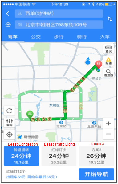
Driving navigation is a core scenario of digital maps. When a user is planning the navigation, AMAP provides three routes for the user to choose from, which are designed based on different factors such as the number of traffic lights.

For most users, the estimated time of arrival (ETA) is a key factor of consideration when selecting a route. And this means that a higher ETA accuracy brings better travel experience for our users. After a user specifies the starting location and the destination, the AMAP app needs to provide a predicted ETA accurately and in real time, which poses significant technical challenges to the AMAP team. In order to achieve this, the team at AMAP employs deep learning based models to predict the flow of traffic based on current and historical data. The following sections will explore these data models and the overall design approach used by AMAP to tackle this challenge.
Traditional machine learning models that are often used for ETA calculation are mainly regression models such as linear regression, Random Forest (RF), and Gradient Boosting Decision Tree (GBDT). Linear models are less expressive, requiring a large amount of feature engineering analysis to get effective features in advance. RF introduces more randomness through sample and feature randomness and solves the problem of weak generalization of decision trees. GBDT achieves regression by using an additive model (linear combination of basis functions) and continuously reducing the residual generated in the training process.
Traditional machine learning models are simpler and easier to understand, and can also achieve good results. However, they have two problems:
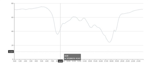
The first problem is easy to understand and can be properly solved by deep learning models. We will illustrate the second problem with the uncertainty in selecting historical speed information as an example. Historical speed information is a historical average time in a 10-minute interval and is specific to the seven days of a week. It can be selected based on the 10-minute interval which contains the estimated point in time when the user enters the road section. The curve in the following figure represents the change of historical average speed over the time period from 00:00 to 24:00, with the value fluctuating greatly during morning and evening rush hours.

The historical average time is selected based on the estimated time of entry, which in turn is dependent on the estimated travel time of the upstream road section. Therefore, the historical average time that will be selected is uncertain, which leads to inaccurate ETA.
In view of this problem, we concatenate all road sections in a route based on the idea of time series in Recurrent Neural Networks (RNNs) to predict the ETA of the route.
Considering the long-term dependency learning problem with RNN and the actual situation of the service, we further choose to use a Long Short Term Memory (LSTM) model for modeling. Additionally, the selectivity offered by the gates in LSTM enables the model to learn on its own to decide which upstream features to retain for prediction.

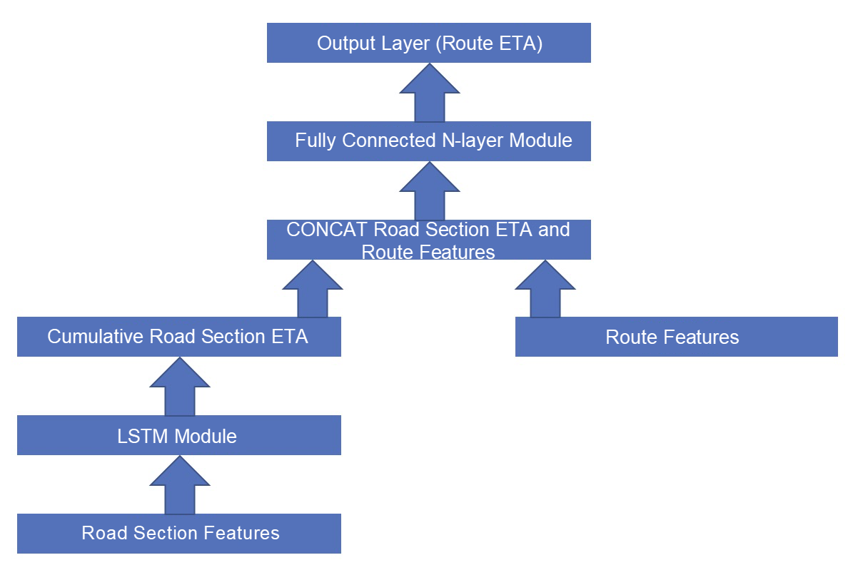
The preceding figure shows the framework of the model, which consists of two parts. The LSTM module is used to predict the ETA of the road sections in the route and finally the fully connected N-layer module is used to predict the ETA of the entire route based on the cumulative road section ETA and features of the route.

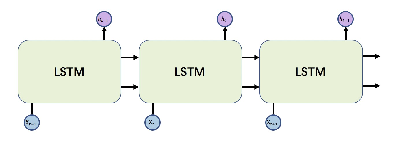
The preceding figure shows the LSTM structure for predicting section ETAs. Xt is the feature information of the t-th road section in the route, including real-time traffic, historical traffic, and static characteristics of the road section.
The LSTM model takes time series as input for prediction. Based on this idea, we input each road section in the route into the model in sequence.
After the LSTM module gets the predicted value of the cumulative road section ETA, the fully connected N-layer module integrates this value with the static properties of the route to output the predicted value of the route ETA.
Property features of a route are manually extracted features that are used to make the model more expressive in different scenarios. They include length of the route, the feature date of the navigation planning, and whether in morning or evening rush hours.
The loss function is the Mean Squared Error (MSE) function, a common square form of linear regression. The formula is as follows:

In the formula, N is the number of routes, ETA Route j is the route ETA, which is the predicted value, and User Travel Time j is the length of time actually spent to travel the route by the user, which is the actual value.
To evaluate the performance of the model, which is the predicted route ETA, we mainly consider the accuracy. Generally, users have higher tolerance for longer ETAs than shorter ones. For example, if a user wants to go to the airport, a predicted ETA that is 10 minutes shorter than the actual time might do more harm to the user than a predicted ETA that is 10 minutes longer. Therefore, the metric for accuracy is designed to favor longer ETAs, which is defined as the ratio of requests that meet a certain range of user tolerance, that is, accuracy is used as the major metric for evaluation.
The experimental results in Beijing show that ETA accuracy is significantly improved with a MSE loss decrease by 28.2%.
This article describes how to build a model for predicting ETA during navigation planning by introducing a deep learning model to resolve the deficiencies of linear models. It also makes room for introducing more features and exploring more possibilities in the future, such as the uncertainty of historical speed information, timeliness, periodicity, emergencies, and road network structure.
amap_tech - December 4, 2019
Alibaba Clouder - June 17, 2020
amap_tech - March 23, 2021
amap_tech - November 20, 2019
amap_tech - November 11, 2019
amap_tech - August 27, 2020
 Platform For AI
A platform that provides enterprise-level data modeling services based on machine learning algorithms to quickly meet your needs for data-driven operations.
Learn More Epidemic Prediction Solution
This technology can be used to predict the spread of COVID-19 and help decision makers evaluate the impact of various prevention and control measures on the development of the epidemic.
Learn More Online Education Solution
This solution enables you to rapidly build cost-effective platforms to bring the best education to the world anytime and anywhere.
Learn More Accelerated Global Networking Solution for Distance Learning
Alibaba Cloud offers an accelerated global networking solution that makes distance learning just the same as in-class teaching.
Learn MoreMore Posts by amap_tech