Sparse vectors store only non-zero values, making them efficient for high-dimensional data where most dimensions are zero — such as keyword-based text representations generated by BM25. This guide covers how to create sparse vector tables and indexes, import data, run exact and approximate searches, and combine sparse with dense vectors for hybrid search.
When to use sparse vectors
| Sparse vectors | Dense vectors | |
|---|---|---|
| Data representation | Most values are zero; only a few dimensions are non-zero | All dimensions have non-zero values |
| Computational efficiency | Higher, especially for zero-element operations | Lower, since all elements are processed |
| Information density | Focuses on key features | Captures nuanced semantic relationships |
| Typical use cases | Keyword search (BM25), hybrid search | Semantic search, RAG, general machine learning |
Use sparse vectors when your data is naturally sparse — for example, when each document is represented as a term-frequency vector over a large vocabulary. Most dimensions will be zero, and only the terms that appear in the document have non-zero values.
Prerequisites
Before you begin, ensure that you have:
An AnalyticDB for PostgreSQL instance running V6.6.2.3 or later. See Create an instance.
The vector search engine optimization feature enabled on the instance. See Enable or disable vector search engine optimization.
How it works
Sparse vectors in AnalyticDB for PostgreSQL use the SVECTOR (Sparse Vector) data type. Instead of storing all dimensions, SVECTOR stores only the non-zero dimensions using a JSON format with two fields:
indices: the positions (non-negative integers) of non-zero valuesvalues: the corresponding floating-point values
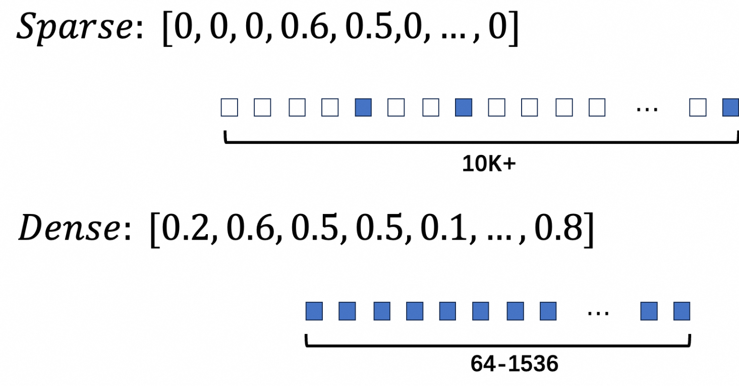
For example, the 20-dimensional vector [0, 0, 1.1, 0, 0, 0, 2.2, 0, 0, 3.3, 0, ...] is stored as:
{"indices":[2, 6, 9], "values":[1.1, 2.2, 3.3]}The figure below shows the structural difference between dense and sparse vectors.
Use sparse vectors
The typical workflow has four steps: create a table, create indexes, import data, and run searches.
Step 1: Create a sparse vector table
CREATE TABLE <table_name> (
    id int PRIMARY KEY,
    description text,
    sparse_vector svector(<MAX_DIM>)
) DISTRIBUTED BY (id);

-- Set the storage mode of the sparse vector column to PLAIN.
ALTER TABLE <table_name> ALTER COLUMN sparse_vector SET STORAGE PLAIN;
Parameters:
| Parameter | Description |
|---|---|
<table_name> | Name of the sparse vector table |
<MAX_DIM> | Maximum number of dimensions, not the count of non-zero values |
Why PLAIN storage? PostgreSQL uses The Oversized-Attribute Storage Technique (TOAST) to store large field values. PLAIN mode disables TOAST compression and splitting, keeping each vector in a single row without being moved to an external table. This avoids the overhead that TOAST introduces for sparse vector access patterns.
Example:
-- Create a table with a sparse vector column.
CREATE TABLE svector_test (
    id bigint,
    type int,
    tag varchar(10),
    document text,
    sparse_features svector(250000)
) DISTRIBUTED BY (id);

-- Set PLAIN storage to prevent TOAST overhead.
ALTER TABLE svector_test ALTER COLUMN sparse_features SET STORAGE PLAIN;
Step 2: Create indexes
Sparse vector indexes have two constraints:
Distance metric: inner product (IP) only — do not use other metrics to avoid errors
No support for product quantization (PQ) or memory mapping
-- Create B-tree indexes for structured columns used in filtered search.
CREATE INDEX ON svector_test (type);
CREATE INDEX ON svector_test (tag);

-- Create an HNSW (Hierarchical Navigable Small World) index on the sparse vector column.
-- DISTANCEMEASURE must be IP (inner product). Using other metrics causes errors.
-- pq_enable=0 and external_storage=0 are required for sparse vectors.
CREATE INDEX ON svector_test USING ANN (sparse_features)
WITH (DISTANCEMEASURE=IP, HNSW_M=64, pq_enable=0, external_storage=0);
For HNSW_M and HNSW_EF_CONSTRUCTION tuning, see Create a vector index.
Step 3: Import sparse vector data
Use INSERT or COPY to load data. Cast the JSON string to svector using ::svector.
-- Insert rows with sparse vector values.
INSERT INTO svector_test VALUES (1, 1, 'a', 'document one',
    '{"indices":[2, 6, 9], "values":[1.1, 2.2, 3.3]}'::svector);
INSERT INTO svector_test VALUES (2, 2, 'b', 'document two',
    '{"indices":[50, 100, 200], "values":[2.1, 3.2, 4.3]}'::svector);
INSERT INTO svector_test VALUES (3, 3, 'b', 'document three',
    '{"indices":[150, 60, 90], "values":[5, 1e3, 1e-3]}'::svector);
To verify the cast:
SELECT '{"indices":[2, 6, 9], "values":[1.1, 2.2, 3.3]}'::svector;
-- Output: {"indices":[2,6,9],"values":[1.1,2.2,3.3]}
Step 4: Search sparse vectors
Choose between exact search and approximate search based on your precision and latency requirements:
| Exact search | Approximate search | |
|---|---|---|
| Algorithm | Brute-force comparison of all vectors | HNSW index traversal |
| Recall rate | Up to 100% | Somewhat reduced |
| Speed | Slower | Faster |
| Use when | Precision is critical; dataset is small | Low latency is required; some precision loss is acceptable |
Exact search
Exact search compares every vector in the table. Use negative_inner_product in the ORDER BY clause to rank results by descending inner product score.
SELECT id,
       inner_product(sparse_features,
           '{"indices":[2,60,50], "values":[2, 0.01, 0.02]}'::svector) AS score
FROM svector_test
ORDER BY negative_inner_product(sparse_features,
    '{"indices":[2,60,50], "values":[2, 0.01, 0.02]}'::svector)
LIMIT 3;
Approximate search
Approximate search uses the HNSW index. Replace negative_inner_product in ORDER BY with the <#> operator to trigger index-based retrieval.
SELECT id,
       sparse_features,
       '{"indices":[2,60,50], "values":[2, 0.01, 0.02]}' <#> sparse_features AS score
FROM svector_test
ORDER BY score
LIMIT 3;
Example output:
 id |                 sparse_features                 |        score
----+-------------------------------------------------+---------------------
  3 | {"indices":[60,90,150],"values":[1000,0.001,5]} |                 -10
  1 | {"indices":[2,6,9],"values":[1.1,2.2,3.3]}      |   -2.20000004768372
  2 | {"indices":[50,100,200],"values":[2.1,3.2,4.3]} | -0.0419999957084656
(3 rows)Adjust recall rate for approximate search using fastann.sparse_hnsw_max_scan_points and fastann.sparse_hnsw_ef_search. See Engine parameters for details.
Hybrid search
Hybrid search combines sparse and dense vectors to improve retrieval quality — sparse vectors capture keyword relevance while dense vectors capture semantic meaning.
Create the hybrid search table and indexes
-- Create a table with both dense and sparse vector columns.
CREATE TABLE IF NOT EXISTS hybrid_search_test (
    id integer PRIMARY KEY,
    corpus text,
    filter integer,
    dense_vector float4[],
    sparse_vector svector(250003)
) DISTRIBUTED BY (id);

-- Set PLAIN storage for both vector columns.
ALTER TABLE hybrid_search_test ALTER COLUMN dense_vector SET STORAGE PLAIN;
ALTER TABLE hybrid_search_test ALTER COLUMN sparse_vector SET STORAGE PLAIN;
-- Structured index for filter pushdown.
CREATE INDEX ON hybrid_search_test (filter);
-- Dense vector HNSW index (DIM=1024, inner product, external storage enabled).
CREATE INDEX ON hybrid_search_test USING ANN (dense_vector)
WITH (DISTANCEMEASURE=IP, DIM=1024, HNSW_M=64, HNSW_EF_CONSTRUCTION=600, EXTERNAL_STORAGE=1);
-- Sparse vector HNSW index (inner product only, no external storage).
CREATE INDEX ON hybrid_search_test USING ANN (sparse_vector)
WITH (DISTANCEMEASURE=IP, HNSW_M=64, HNSW_EF_CONSTRUCTION=600);Run search queries
All three examples below use FILTER IN (...) for pre-filtering results by a structured column before vector ranking.
-- Dense vector search with filter.
SELECT id, corpus
FROM hybrid_search_test
WHERE filter IN (0, 100, 200, 300, 400, 500, 600, 700, 800, 900)
ORDER BY dense_vector <#> ARRAY[1,2,3,...,1024]::float4[]
LIMIT 100;

-- Sparse vector search with filter.
SELECT id, corpus
FROM hybrid_search_test
WHERE filter IN (0, 100, 200, 300, 400, 500, 600, 700, 800, 900)
ORDER BY sparse_vector <#> '{"indices":[1,2,..], "values":[1.1,2.2...]}'::svector
LIMIT 100;

-- Hybrid search with filter.
-- Strategy: retrieve the top 100 candidates from each index independently,
-- then re-rank by combining both distance scores (dist1 - dist2).
-- This avoids score-scale incompatibility between sparse and dense distances.
-- Using MAX(dist1 - dist2) per id deduplicates candidates from the UNION ALL.
WITH combined AS (
    -- Branch 1: top 100 by sparse score.
    -- dist1 = dense distance (secondary signal for re-ranking).
    -- dist2 = sparse distance (primary retrieval signal for this branch).
    (SELECT id, corpus,
            inner_product_distance(dense_vector, ARRAY[1,2,3,...,1024]::float4[]) AS dist1,
            sparse_vector <#> '{"indices":[1,2,..], "values":[1.1,2.2...]}'::svector AS dist2
     FROM hybrid_search_test
     WHERE filter IN (0, 100, 200, 300, 400, 500, 600, 700, 800, 900)
     ORDER BY dist2 LIMIT 100)
    UNION ALL
    -- Branch 2: top 100 by dense score.
    -- dist1 = sparse distance (secondary signal for re-ranking).
    -- dist2 = dense distance (primary retrieval signal for this branch).
    (SELECT id, corpus,
            inner_product(sparse_vector, '{"indices":[1,2,..], "values":[1.1,2.2...]}'::svector) AS dist1,
            dense_vector <#> ARRAY[1,2,3,...,1024]::float4[] AS dist2
     FROM hybrid_search_test
     WHERE filter IN (0, 100, 200, 300, 400, 500, 600, 700, 800, 900)
     ORDER BY dist2 LIMIT 100)
)
SELECT DISTINCT
    first_value(id) OVER (PARTITION BY id) AS id,
    first_value(corpus) OVER (PARTITION BY id) AS corpus,
    MAX(dist1 - dist2) OVER (PARTITION BY id) AS dist
FROM combined
ORDER BY dist DESC
LIMIT 100;
Appendix
Engine parameters
Both parameters apply per session. Use them to tune the trade-off between recall rate and query speed for approximate sparse vector search.
| Parameter | Description | Default | Valid range |
|---|---|---|---|
fastann.sparse_hnsw_max_scan_points | Maximum number of scan points during HNSW sparse vector search. Lower values terminate search earlier, trading recall for speed. | 8000 | [1, 8000000] |
fastann.sparse_hnsw_ef_search | Size of the search candidate set during HNSW traversal. Higher values increase recall but slow down queries. | 400 | [10, 10000] |
Supported functions
All functions below operate on the SVECTOR data type.
| Function | Return type | Description |
|---|---|---|
l2_distance | DOUBLE PRECISION | Euclidean (L2) distance between two sparse vectors |
inner_product | DOUBLE PRECISION | Inner product; equivalent to cosine similarity after vector normalization |
dp_distance | DOUBLE PRECISION | Dot product distance; same as inner_product |
cosine_similarity | DOUBLE PRECISION | Cosine similarity; range: -1 to 1 |
svector_add | SVECTOR | Element-wise sum of two sparse vectors |
svector_sub | SVECTOR | Element-wise difference between two sparse vectors |
svector_mul | SVECTOR | Element-wise product of two sparse vectors |
svector_norm | DOUBLE PRECISION | L2 norm of a sparse vector |
svector_angle | DOUBLE PRECISION | Angle between two sparse vectors |
l2_squared_distance | DOUBLE PRECISION | Squared Euclidean distance; faster than l2_distance for sorting |
negative_inner_product | DOUBLE PRECISION | Negative inner product; use in ORDER BY to sort by descending inner product |
cosine_distance | DOUBLE PRECISION | Cosine distance; range: 0 to 2 |
Examples:
-- Euclidean distance
SELECT l2_distance(
    '{"indices":[1,2,3,4,5,6], "values":[1,2,3,4,5,6]}'::svector,
    '{"indices":[1,2,3,4,5,6], "values":[2,3,4,5,6,7]}'::svector);

-- Inner product
SELECT inner_product(
    '{"indices":[1,2,3,4,5,6], "values":[1,2,3,4,5,6]}'::svector,
    '{"indices":[1,2,3,4,5,6], "values":[2,3,4,5,6,7]}'::svector);

-- Cosine similarity
SELECT cosine_similarity(
    '{"indices":[1,2,3,4,5,6], "values":[1,2,3,4,5,6]}'::svector,
    '{"indices":[1,2,3,4,5,6], "values":[2,3,4,5,6,7]}'::svector);

-- Vector arithmetic
SELECT svector_add(
    '{"indices":[1,2,3,4,5,6], "values":[1,2,3,4,5,6]}'::svector,
    '{"indices":[1,2,3,4,5,6], "values":[2,3,4,5,6,7]}'::svector);

SELECT svector_sub(
    '{"indices":[1,2,3,4,5,6], "values":[1,2,3,4,5,6]}'::svector,
    '{"indices":[1,2,3,4,5,6], "values":[2,3,4,5,6,7]}'::svector);

SELECT svector_mul(
    '{"indices":[1,2,3,4,5,6], "values":[1,2,3,4,5,6]}'::svector,
    '{"indices":[1,2,3,4,5,6], "values":[2,3,4,5,6,7]}'::svector);

-- Sorting functions
SELECT l2_squared_distance(
    '{"indices":[1,2,3,4,5,6], "values":[1,2,3,4,5,6]}'::svector,
    '{"indices":[1,2,3,4,5,6], "values":[2,3,4,5,6,7]}'::svector);

SELECT negative_inner_product(
    '{"indices":[1,2,3,4,5,6], "values":[1,2,3,4,5,6]}'::svector,
    '{"indices":[1,2,3,4,5,6], "values":[2,3,4,5,6,7]}'::svector);

SELECT cosine_distance(
    '{"indices":[1,2,3,4,5,6], "values":[1,2,3,4,5,6]}'::svector,
    '{"indices":[1,2,3,4,5,6], "values":[2,3,4,5,6,7]}'::svector);
Supported operators
All operators below work with the SVECTOR type.
| Operator | Calculation | Sorting behavior |
|---|---|---|
<-> | Squared Euclidean distance (equivalent to l2_squared_distance) | Not supported |
<#> | Negative inner product (equivalent to negative_inner_product) | Sorts in descending order by dot product |
<=> | Cosine distance (equivalent to cosine_distance) | Not supported |
+ | Element-wise sum | Not supported |
- | Element-wise difference | Not supported |
* | Element-wise product | Not supported |
Examples:
-- Squared Euclidean distance
SELECT '{"indices":[1,2,3,4,5,6], "values":[1,2,3,4,5,6]}'::svector
    <-> '{"indices":[1,2,3,4,5,6], "values":[2,3,4,5,6,7]}'::svector AS score;

-- Negative inner product (use in ORDER BY for approximate search)
SELECT '{"indices":[1,2,3,4,5,6], "values":[1,2,3,4,5,6]}'::svector
    <#> '{"indices":[1,2,3,4,5,6], "values":[2,3,4,5,6,7]}'::svector AS score;

-- Cosine distance
SELECT '{"indices":[1,2,3,4,5,6], "values":[1,2,3,4,5,6]}'::svector
    <=> '{"indices":[1,2,3,4,5,6], "values":[2,3,4,5,6,7]}'::svector AS score;

-- Vector arithmetic
SELECT '{"indices":[1,2,3,4,5,6], "values":[1,2,3,4,5,6]}'::svector
    + '{"indices":[1,2,3,4,5,6], "values":[2,3,4,5,6,7]}'::svector AS value;

SELECT '{"indices":[1,2,3,4,5,6], "values":[1,2,3,4,5,6]}'::svector
    - '{"indices":[1,2,3,4,5,6], "values":[2,3,4,5,6,7]}'::svector AS value;

SELECT '{"indices":[1,2,3,4,5,6], "values":[1,2,3,4,5,6]}'::svector
    * '{"indices":[1,2,3,4,5,6], "values":[2,3,4,5,6,7]}'::svector AS value;