Learning Stable Graphs from Heterogeneous Confounded Environments

Download the "Cloud Knowledge Discovery on KDD Papers" whitepaper to explore 12 KDD papers and knowledge discovery from 12 Alibaba experts.

By Yue He, Peng Cui, Jianxin Ma, Hao Zou, Xiaowei Wang, Hongxia Yang, Philip S. Yu

Background

Graphs can be used to describe the universal relations between things, which can be encoded into parameterized graph structures, such as an adjacency matrix. Expert-based graph composition methods require costly, manually collected information. It is difficult to deploy the composed graphs in a wide range of production and daily life environments. This boosts the research on data-driven graph generation algorithms. A data-driven graph generation algorithm is intended to compose a graph that can best describe the input data generation process. For example, in a recommendation scenario, the input data can be a buyer's shopping records, and a product network graph expresses the intensity of relations between items. Data-driven algorithms rely heavily on the conditional independence assumption of data. This assumption prescribes that training scenarios and test scenarios have the same data distribution. If this assumption is not satisfied, graph performance is significantly decreased. In reality, the independence assumption is very fragile. The data sampling process is subject to temporal and spatial limitations. For example, among online shoppers, women usually account for a larger proportion than men, and young people account for a larger proportion than elderly people. The graph that is learned based on this fact shows much more preferences for young women than for other groups. Therefore, it makes sense to improve the generalization performance of graph structures.

Challenges

By learning cause-and-effect diagrams, we can directly capture the constant causal relations between things to guarantee stability. However, learning of cause-and-effect diagrams requires highly complex computations, and it is difficult to apply the learning process to large networks. Moreover, cause-and-effect diagrams are a type of directed acyclic graph (DAG) and unable to describe extensive, scenario-based cyclic structures. Graph structures contain complex high-order, nonlinear relations. This makes it difficult to correct deviations directly in the original graph structure space, such as an adjacency matrix. In addition, the input data used to generate graph structures is high-dimensional and sparse, such as the set data type. This paper presents the SGL, a method used to learn stable, generic graph structures in heterogeneous confounded environments.

Model

To suit more general scenarios, we assume that the input data is of the set type, which is high-dimensional and sparse. The generation of a set data record can be viewed as the process of adding elements to an empty set one by one until the set is saturated. For the mth data environment, the probability of adding each element IkIk to a given set s is equal to the conditional generative probability p(m)(Ik|s)p(m)(Ik|s) of the set. Obviously, pm (I_k│s) pm (I_k│s) is related to the element relations contained in the graph structure G(m)G(m) and can be expressed as follows:

The conditional generative probability is biased due to sampling deviations in various heterogeneous environments. Assume that the environment selection is random. The probability space of each environment on average is the estimation of an unbiased environment.

A graph structure is full of high-order, nonlinear relations. This makes it difficult to eliminate deviations directly in the parameter space (adjacency matrix) of the graph structure. However, we can indirectly correct these deviations if we can establish a mapping from the graph structure to the conditional generative probability and balance the deviations in the generation probability space.

Graph-based Sparse Set Generation

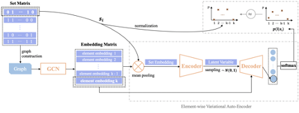
According to the preceding ideas, the first thing to do is to establish a mapping from the graph structure to the conditional generative probability. Given that different biased data environments exist, we can first use a method based on joint occurrence frequencies to create an initial graph in each environment, with each point representing an element in a set. The SGL framework consists of two modules. The first module is a graph convolutional neural network, which embeds the structural features of the initial graph into the output element representations. By pooling all the element representations of a set, we can acquire the feature vectors of this set. The feature vectors are passed to the second module, the element-level variational autoencoder (E-VAE). This module reconstructs the real data and learns the set generation probability. We can acquire a hidden space distribution by processing the feature vectors of the set with an encoder. We can also sample a hidden vector from the encoded vectors and decode this hidden vector in conjunction with the representation of each element. This results in the intensity of each element to be included into the set. Then, we project the intensities of all elements to the probability space to output the set generation probability. Assume that the input set is saturated. We can reconstruct raw data to learn the conditional generative probability space in an environment. In other words, we want to apply conditions to the output probability of real samples. After we add new sampled elements, we keep the set unchanged to maximize the occurrence probability of real samples.

Considering the sparsity of set data, we use the negative log likelihood function as an objective function to optimize model learning.

We also optimize the Kullback-Leibler (KL) divergence between the hidden distribution and the predefined normal distribution in the E-VAE as follows:

Learning a Stable Graph Structure

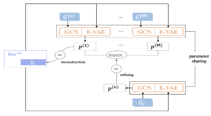
By training graph convolutional networks (GCNs) and E-VAEs that share the same parameters in each environment, we can acquire the conditional generative probabilities for the same input set in different environments. Assume that we are initializing the graph structure of an unbiased data environment. We can optimize this graph structure so that the generation probability of the unbiased environment that is output by this graph is the average of the generation probabilities of all biased environments. This can produce a stable graph structure.

Considering the interactions between various parts, we jointly optimized the adjacency matrix of the GCNs, E-VAEs, and stable graph structures. Optimized with the SGD framework, the model is applicable to graphs of more sizes.

Experiments

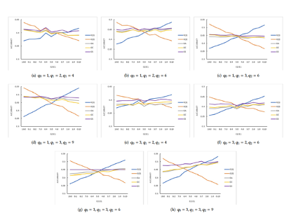
To verify the effectiveness of the model, we conducted experiments on simulated data and real data, respectively. In the simulated data experiment, we used a biased random walk to generate walk paths with different data distributions in two environments. The random walk used p_0 (zero-order correlations, such as users' prior preferences), p_1 (first-order correlations of elements), and p_2 (second-order correlations of elements) to control the degree of differences between the two environments. The distribution differences were proportional to the values of p_0, p_1, and p_2. Then, we used the training data in each environment to create a graph based on joint occurrence frequencies. This way, we acquired two graphs with different implicit relations.

The frequency diagrams G1 and G2 were created for the two environments, respectively. Our baseline model applied the equation GA=(G1+G2)/2 and mixed the data of the two environments evenly and proportionally to compose the frequency diagram GC. Based on G1, G2, and training data, we learned the stable graph structure GS.

To test the stability of different graph structures, we designed a set prediction task. First, we divided a test set into target elements and remaining known elements. Given the element representations learned from graph structures and the known elements of the test set, we aimed to select the target elements from all candidate nodes, that is, to select the elements closest to the remaining elements of the set. Then, we mixed the test data of the two environments with 0:10, 1:9, ..., and 10:0 ratios to get 11 test groups. We collected statistics on the element representations learned from different graph structures. We used the average COS distance between the element representations to measure the prediction accuracy in multiple test groups with different data distributions. To ensure the fairness of experiments, we used the same GCN to learn the element representations of different graphs.

According to the following results, the applicability of intra-graph relations in a single environment diminishes with the increase of data in another environment. The intra-graph nonlinear relations are not considered when the linear average of graphs in each environment is calculated. The approach of graph composition by mixing data in various environments is not immune to the model deviations that are inherent in a traditional graph composition method. This approach also cannot solve the zero-order correlation problem, such as differences between users' prior preferences. A stable graph structure can be used to achieve the optimal prediction accuracy with the minimum standard deviation. The reason is that this graph can balance the deviations of high-order, nonlinear relations in different test environments.

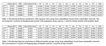
The real data experiment was conducted in two scenarios: differences between user populations and exposure differences between various products. The first scenario involves the different proportions of various user populations. The second scenario involves the different popularities of dominant products in different environments. For the differences between user populations, we divided male and female users into two environments. For the exposure differences between various products, we first identified popular products. Then, we divided all shopping records into a popular-dominant environment and an unpopular-dominant environment based on whether the proportion of popular products in each of these records exceeds 50%. The experiments used to verify the baseline model and prediction tasks are the same as the simulated data experiment.

The experiment results show that the prediction difficulty varies depending on different environments. It is easier to predict the shopping behavior of women than men. This is probably because women are more interested in a highly correlated product than men. In addition, prediction is easier for shopping records that contain many popular products. This is probably because popular products are more highly correlated with each other. SGL can learn more generic information from different environments to achieve the optimal prediction rate.

Summary

We present the SGL learning framework to learn stable graph structures from heterogeneous confounded environments. By generating sparse data based on graphs, the framework establishes a mapping from the graph structure to the generation probability space. It then balances biased information in the generation probability space to correct the structural deviations of graphs. Experiments show that our method can improve the stability of graph structures and provide effective solutions to practical problems.

Reference

[1] Lada A Adamic and Eytan Adar. 2003. Friends and neighbors on the web. Social networks 25, 3 (2003), 211-230.
[2] Aleksandar Bojchevski, Oleksandr Shchur, Daniel Zügner, and Stephan Günnemann. 2018. Netgan: Generating graphs via random walks. arXiv preprint arXiv:1803.00816 (2018).
[3] Peter Bühlmann, Jonas Peters, Jan Ernest, et al. 2014. CAM: Causal additive models, high-dimensional order search and penalized regression. The Annals of Statistics 42, 6 (2014), 2526-2556.
[4] Abhishek Gupta, Coline Devin, YuXuan Liu, Pieter Abbeel, and Sergey Levine. 2017. Learning invariant feature spaces to transfer skills with reinforcement learning. arXiv preprint arXiv:1703.02949 (2017).
[5] Kilol Gupta, Mukund Yelahanka Raghuprasad, and Pankhuri Kumar. [n.d.]. A Hybrid Variational Autoencoder for Collaborative Filtering. ([n. d.]).
[6] Bo Jiang, Ziyan Zhang, Doudou Lin, Jin Tang, and Bin Luo. 2019. Semi-supervised learning with graph learning-convolutional networks. In Proceedings of the IEEE Conference on Computer Vision and Pattern Recognition. 11313-11320.
[7] Diederik P Kingma and Max Welling. 2013. Auto-encoding variational bayes. arXiv preprint arXiv:1312.6114 (2013).

The views expressed herein are for reference only and don't necessarily represent the official views of Alibaba Cloud.

Community

Learning Stable Graphs from Heterogeneous Confounded Environments

Background

Challenges

Model

Graph-based Sparse Set Generation

Learning a Stable Graph Structure

Experiments

Summary

Reference

Read previous post:

Read next post:

Alibaba Clouder

You may also like

Comments

Alibaba Clouder

Related Products

Platform For AI

Epidemic Prediction Solution

Machine Translation

Online Education Solution