Classic Supervised Learning Algorithm-Decision Tree

By Bailuo, from F(x) Team

As one of the classic Machine Learning algorithms, decision trees (including algorithms derived from or used as the smallest decision unit, including random forests, slope climbing trees, XGBoost, etc.) are prevalent in neural networks today. Also, it still has an important position in the supervised learning algorithm family.

It is a Machine Learning prediction model that provides decision-making capabilities based on a tree model. Each node in the tree represents an object, and the corresponding fork path represents its property value. The leaf node corresponds to the value of the object represented by the path from the root node to the leaf node. The following section will show how a basic decision tree model works through a classic example based on the basic principles and the principles of the decision tree.

1. Empirical Risk Minimization

There are often the following training sets and objectives for supervised learning tasks: training set: S = {(X1, y1), ..., (Xn, yn)} target: h: X->y mapping, which can perform well in the actual task t. (h indicates hypothesis.)

We do not know how the model will operate in a real-world scenario, but we usually verify the performance of the model on a set of marked training sets.

Empirical Risk Minimization Principle: The ultimate goal of the Machine Learning algorithm is to find a hypothesis with the smallest average loss function on the data set (i. e. the smallest risk) in a set of hypotheses:

R(h) = E(L(h(x), y)) E denotes expectation and L denotes loss function

It is based on the premise that the training set is sufficiently representative of the real situation. It is known that the training set is often not representative of the real situation, the result is the overfitting of the model, which is similar to the difference between the exercise with the answer and the final exam.

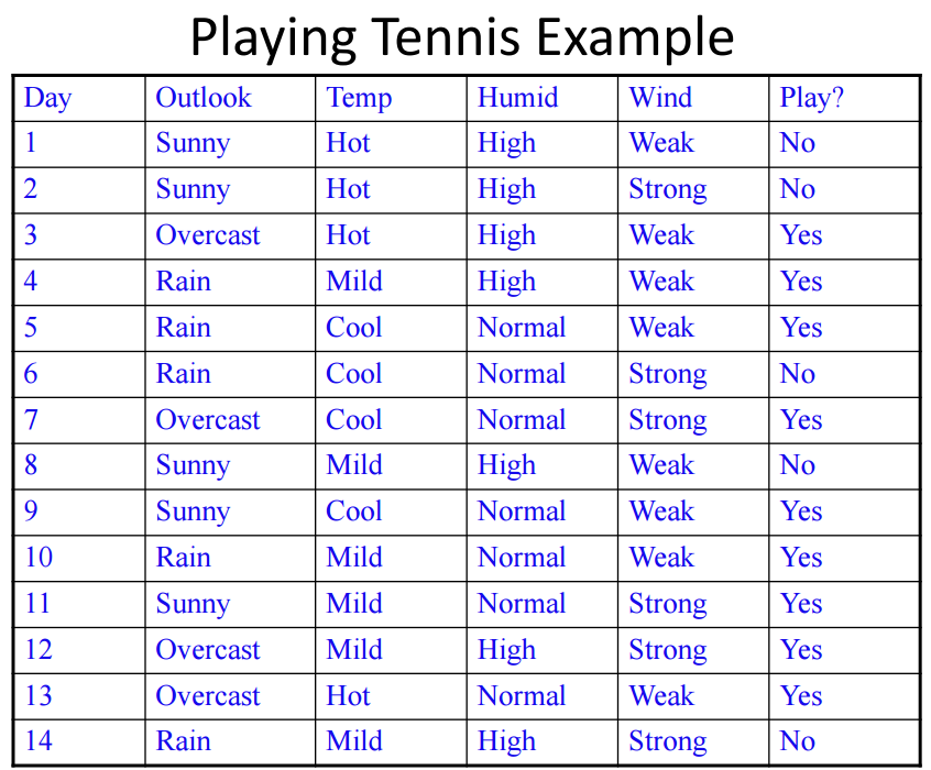
2. Algorithm Theory of Decision Tree

A decision tree is a directed acyclic graph characterized by each non-leaf node being associated with an attribute. The edge represents the value of the parent node of the attribute, while leaf nodes are associated with the label. Here, we can use a classic example to understand the basic principles of the decision tree algorithm. The following is a training set for weather conditions and deciding whether to play tennis. (This is a four-dimensional input and one-dimensional output.)

Outlook has Sunny, Overcast, and Rain in this data set. Temp has Hot, Mild, and Cold. Humid has High and Normal. Wind has Weak and Strong. Therefore, there are a total of 3x3x2x2=36 combinations, each of which corresponds to both Yes and No predictions. If we want to build a model of a decision tree, there will be a total of 236 different hypotheses. Which of them will be the most appropriate model is the next question that will be discussed.

2.1 Ockham's Razor

In the preceding section, we pointed out 236 different decision tree models for this training set. How many of these possible models can do the right prediction model on these 14 samples (the samples are not contradictory to each other)? The answer is 2(36-14) = 222.

William of Ockham (a 13th century English philosopher and Franciscan monk) popularized a classic logic rule: plurality should not be posited without necessity. In other words, all systems should be as simple as possible. This theory can be combined with the empirical risk minimization mentioned earlier and become the cornerstone of decision tree construction design. Since this is an NP-Hard problem, we can use Greedy Procedure-Recursive here to pick out the most concise among the 222 models that can achieve the purpose, starting from the root stage and performing the following loop:

Select a good attribute as the node
According to the value of this attribute (for example, the value of Wind is Strong and Weak) as an edge splits into different child nodes.
If all samples have the same label, this node ends here. (In other words, if all samples have the same labels, there is no need to continue to divide them if they can be summarized with one label.)

2.2 Gini Impurity and Cross Entropy Loss

In the growth strategy of the decision tree, we mentioned the need to select a good attribute as a node at a time. We need to maximize the discrimination of labels by the descendants of that node (reducing the randomness of classification). For example, attribute A grows along with two values of 0 and 1, and the labels of samples on child nodes are (4 Yes, 4 No), (3 Yes, 3 No). Attribute B grows along with two values of 0 and 1, and the sample labels on the child nodes are (8 Yes, 0 No), (0 Yes, 6 No). Then, it is obvious that choosing node B will be more differentiated. There are generally two indicators to quantify this degree of discrimination: Gini Impurity and Information Gain. In principle, the decision tree should grow along the direction where the Gini index or cross entropy loss decreases the fastest.

If the number of tags is distributed as:

n1, n2, ......, nL

The cross entropy loss can be described as:

H(S) = (n1/n) log(n/n1) + (n2/n) log(n/n2) + ...... + (nL/n) log(n/nL)

We can obtain the information gain by the difference between the cross entropy loss of the parent node (S) and the weighted cross entropy loss of the child node (v):

IG(S) = H(S) - (n1/n)H(v1) - (n2/n)H(v2) - ...... - (nL/n)H(vL)

Similarly, the Gini index can be described as:

Gini(S) = 1 - (n1/n)2 - (n2/n)2 - ....... - (nL/n)2

Similarly, the Gini purity can be obtained from the difference between the Gini index of the parent node (S) and the weighted Gini index of the child node (v):

GiniImp(S) = Gini(S) - (n1/n)Gini(v1) - (n2/n)Gini(v2) - ...... - (nL/n)Gini(vL)

If you use the tennis example mentioned earlier, a complete decision tree uses Gini impurity as a decision-making method. Its growth process will look like this. First, at the root node, when no attributes are used, the training set can be divided into (9 Yes, 5 No), and the corresponding Gini index is shown below:

Calculate the Gini impurity with the attributes of the four dimensions as an indicator of decision tree growth, respectively:

The Outlook attribute has the highest degree of impurity, which means that choosing this dimension to grow at this time can distinguish the training set better.

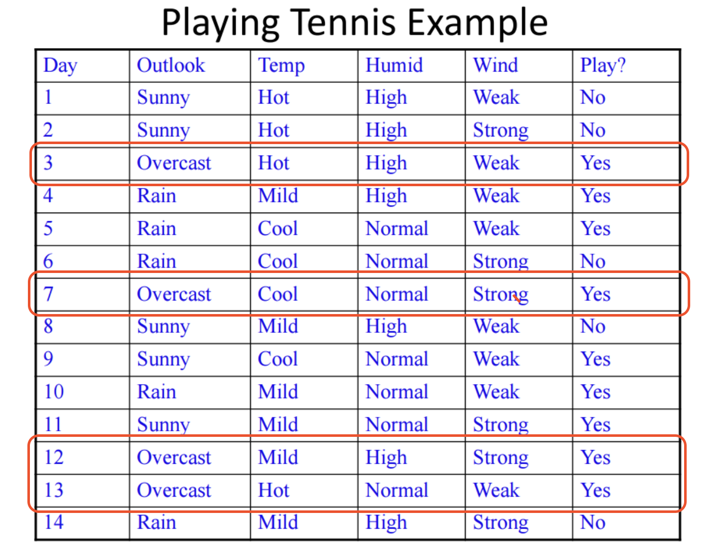
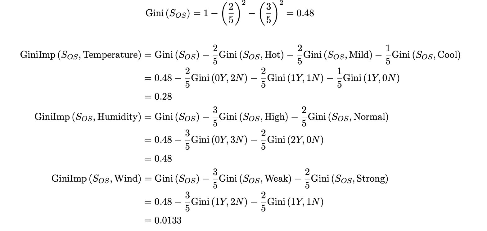
We can observe that when the Outlook value is Overcast, the sample is (4 Yes, 0 No), which means that all branches are correctly classified and can be terminated. If the Sunny attribute is counted as OS and the Rain attribute is counted as OR, the next Gini impurity can be calculated after selecting Outlook - Sunny:

Choosing Humidity can minimize randomness, so the child node of Outlook - Sunny is Humidity. Meanwhile, we observed that all samples can be correctly classified, and this branch can be terminated.

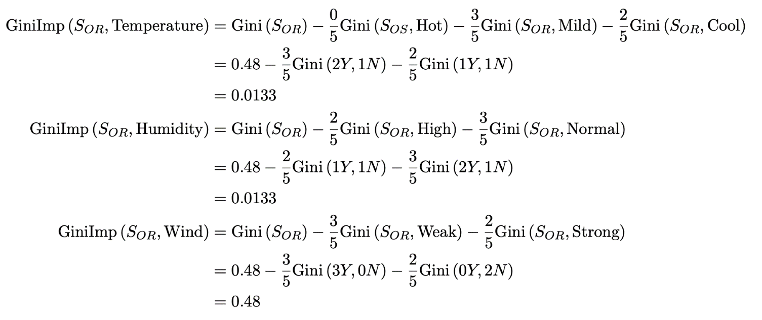
Similarly, for Outlook - Rain, it can be calculated as:

Choosing Wind as a child node minimizes randomness. It is observed that all subsequent samples can be correctly classified, so the branch ends. In summary, we can obtain a decision tree with the following structure, which is a better solution generated by using the recursive greedy strategy (guided by the ERM and Ockham's Razor principles):

3. Overfitting Suppression

The overfitting suppression strategy of the decision tree can generally be divided into prepruning and postpruning. Among them, the prepruning is generally based on preset rules (such as the maximum number of nodes, the maximum height, the impurity of Gini or the growth of information gain, etc.) to stop the growth of the tree in advance. Postpruning is pruning after the tree is fully grown, such as adding penalties to losses based on complexity. In the postpruning process, those branches that are inefficient to Gini impurity or information gains are eliminated.

Community

Classic Supervised Learning Algorithm-Decision Tree

1. Empirical Risk Minimization

2. Algorithm Theory of Decision Tree

2.1 Ockham's Razor

2.2 Gini Impurity and Cross Entropy Loss

3. Overfitting Suppression

Read previous post:

Read next post:

Alibaba F(x) Team

You may also like

Comments

Alibaba F(x) Team

Related Products

Platform For AI

Epidemic Prediction Solution

AI Acceleration Solution

Machine Translation