Areal rainfall analysis using the
GanosBase Raster is a spatio-temporal engine extension for PolarDB for PostgreSQL (Compatible with Oracle). This tutorial walks through a complete areal precipitation analysis pipeline: importing point observation data, interpolating it into a raster grid, generating contour lines and surfaces, collecting statistics, and computing a weighted areal precipitation value — all within the database using SQL.
GanosBase Raster overview
GanosBase Raster stores, manages, and processes raster data types inside the database. It supports data from remote sensing, photogrammetry, and thematic mapping, and can publish raster objects as OGC (Open Geospatial Consortium) standard services such as WMS (Web Map Service) and WMTS (Web Map Tile Service) through a GeoServer extension.
Raster data model
The GanosBase raster data model consists of six elements:
| Element | Description |
|---|---|
| Raster | A raster dataset, such as a remote sensing image or a TIFF file |
| Tile | The basic storage unit of a raster object; defaults to 256 × 256 pixels |
| Band | A single 2D layer in a raster dataset; each band comprises multiple tiles |
| Cell | A pixel in a tile; supported data types include byte, short, int, and double |
| Pyramid | A series of reduced-resolution versions of the raster; Level 0 is the raw data |
| Metadata | Raster attributes including spatial extent, projection type, and pixel type |
A raster object is logically divided into bands, each holding raw image data. Tiles store and manage the data within each band. Each raster object carries its own metadata — spatial extent, data type, projection, and coordinates. If a raster is organized in a pyramid structure, each band has its own pyramid levels.

Raster data categories
Raster data falls into two categories:
-
Thematic data: each pixel value is a measurement or classification — for example, DEM (digital elevation model) data, pollutant concentration, signal strength, precipitation, land ownership, or vegetation types.
-
Remote sensing images: images captured by ground, aerial, or satellite platforms that reflect the electromagnetic characteristics of objects. Because raster data carries both spatial and temporal attributes, it can also manage time series.
Key capabilities
GanosBase Raster uses an object-oriented storage structure: each raster — whether a remote sensing image or a DEM file — is stored as a single database record, with each record supporting up to 1 TB. Direct operations on tiles are not allowed, preserving metadata integrity.
Raster metadata is kept in the database while raster attribute data is stored on OSS (Object Storage Service), significantly reducing storage costs for large-scale image analysis. Beyond standard spatial operations, GanosBase Raster provides statistical and algebraic operations, image color balancing algorithms, and accelerated overview rendering for large raster datasets.
Areal precipitation analysis
Background
Areal precipitation is the average precipitation per unit area within a region. It is a key indicator in flood forecasting, used for flood control, reservoir regulation, and disaster prevention. Because precipitation is typically measured at discrete observation sites, analysis requires spatially interpolating the point measurements into a continuous grid, then computing weighted statistics over the target area.
This tutorial implements the following pipeline:
-
Import point observation data and polygon boundary data using the FDW (Foreign Data Wrapper) extension
-
Interpolate point data into a raster grid using IDW (Inverse Distance Weighting)
-
Generate contour lines and surfaces from the raster
-
Collect interval statistics on precipitation distribution
-
Calculate the weighted areal precipitation for any polygon boundary
Prerequisites
Before you begin, make sure you have:
-
A PolarDB for PostgreSQL (Compatible with Oracle) instance
-
Point observation data and polygon boundary data in ESRI Shapefile format, stored in an OSS bucket
-
Your AccessKey ID (AccessKeyId) and AccessKey Secret (AccessKeySecret)
-
The OSS endpoint and bucket name
Install extensions
Install the ganos_raster and ganos_fdw extensions in your target database:
CREATE EXTENSION ganos_raster CASCADE;
CREATE EXTENSION ganos_fdw CASCADE;
Import data
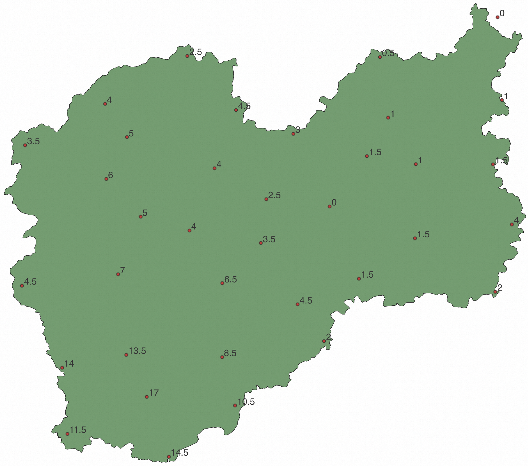
The source data consists of two shapefiles:
-
point.shp— a point layer where each point has anidattribute (string) and apreattribute (precipitation, floating-point) -
polygon.shp— a polygon layer representing the administrative boundary
The following QGIS overlay shows the 36 observation points. Each number is the precipitation value at that location:
Step 1: Create a foreign server and map the shapefiles as external tables.
-- Create a foreign server pointing to the OSS bucket
CREATE SERVER myserver
  FOREIGN DATA WRAPPER ganos_fdw
  OPTIONS (
    datasource 'OSS://<access_id>:<secret_key>@<endpoint>/<bucket>/path_to/file',
    format 'ESRI Shapefile'
  );

CREATE USER MAPPING FOR CURRENT_USER
  SERVER myserver
  OPTIONS (user '<access_id>', password '<access_key_secret>');

-- Map shapefiles as external tables
CREATE FOREIGN TABLE foreign_point_table (
  fid   integer,
  id    varchar,
  geom  geometry,
  pre   double precision  -- precipitation value
)
SERVER myserver
OPTIONS (layer 'point');

CREATE FOREIGN TABLE foreign_polygon_table (
  fid   integer,
  id    varchar,
  geom  geometry
)
SERVER myserver
OPTIONS (layer 'polygon');
Replace the following placeholders:
| Placeholder | Description |
|---|---|
<access_id> |
Your AccessKeyId |
<secret_key> |
Your AccessKeySecret |
<endpoint> |
The OSS endpoint |
<bucket> |
The name of your OSS bucket |
Step 2: Create local tables and insert data from the external tables.
CREATE TABLE point_table   AS SELECT fid, geom, pre FROM foreign_point_table;
CREATE TABLE polygon_table AS SELECT fid, geom      FROM foreign_polygon_table;
Step 3: Verify the imported data.
SELECT fid, ST_AsText(geom), pre FROM point_table;Expected output (36 rows):
 fid  |          st_astext          | pre
------+-----------------------------+------
    0 | POINT(119.1084 28.50302)    |    5
    1 | POINT(118.768925 28.475747) |  3.5
    2 | POINT(119.30954 28.773729)  |  2.5
  ...
   35 | POINT(119.248086 27.435982) | 14.5
(36 rows)
Perform spatial interpolation
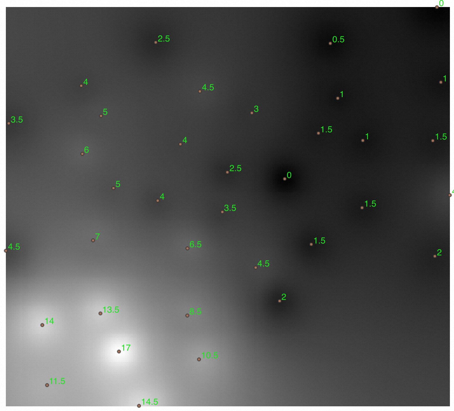
converts point observations into a raster grid using spatial interpolation. This example uses IDW, which estimates each grid cell's value as a weighted average of surrounding points, giving more weight to closer points.
Step 1: Create a table to store the interpolated raster.
CREATE TABLE IF NOT EXISTS raster_table (
  id   integer,
  rast raster  -- stores the interpolated raster object
);
Step 2: Run the interpolation and insert the result.
INSERT INTO raster_table (id, rast)
VALUES (
  1,
  (SELECT ST_InterpolateRaster(
    ST_Collect(ST_MakePoint(ST_X(geom), ST_Y(geom), pre)),  -- input: 3D point collection (x, y, precipitation)
    512,                                                      -- output grid width (pixels)
    512,                                                      -- output grid height (pixels)
    '{"method":"IDW","radius":2.0,"max_points":"30","min_points":"1"}',  -- IDW algorithm options
    '{"chunktable":"rbt","celltype":"32bf"}'                             -- storage options
  )
  FROM point_table)
);
IDW algorithm options:
| Parameter | Description | Value in this example |
|---|---|---|
method |
Interpolation method | IDW |
radius |
Search radius (degrees) for neighboring points | 2.0 |
max_points |
Maximum number of neighboring points used | 30 |
min_points |
Minimum number of neighboring points required | 1 |
When processing large point datasets, enable parallel processing before running the interpolation:
-- Set the degree of parallelism
SET ganos.parallel.degree = 4;
Step 3: Export the raster to verify the result.
exports the raster as a COG (Cloud Optimized GeoTIFF) to OSS:
SELECT ST_ExportTo(
  rast,
  'COG',
  'OSS://<access_id>:<secret_key>@<endpoint>/<bucket>/path_to/output.tif'
)
FROM raster_table
WHERE id = 1;
Open the exported file in QGIS to verify the interpolated surface:
Step 4: Clip the raster to the administrative boundary.
clips the interpolated raster using the polygon from polygon_table, producing a raster that covers only the area of interest:
INSERT INTO raster_table
SELECT 2, ST_ClipToRast(r.rast, p.geom, 0, '', NULL, '', '{"chunktable":"rbt"}')
FROM raster_table AS r, polygon_table AS p;
Export the clipped raster to verify:
SELECT ST_ExportTo(
  rast,
  'COG',
  'OSS://<access_id>:<secret_key>@<endpoint>/<bucket>/path_to/idw_clip.tif'
)
FROM raster_table
WHERE id = 2;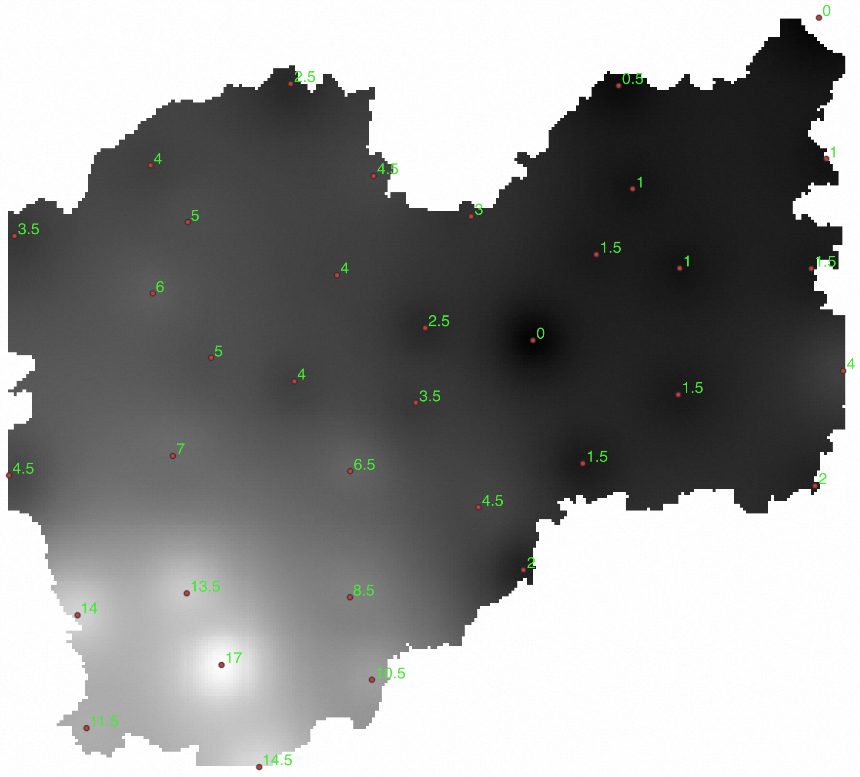
Generate contours and surfaces
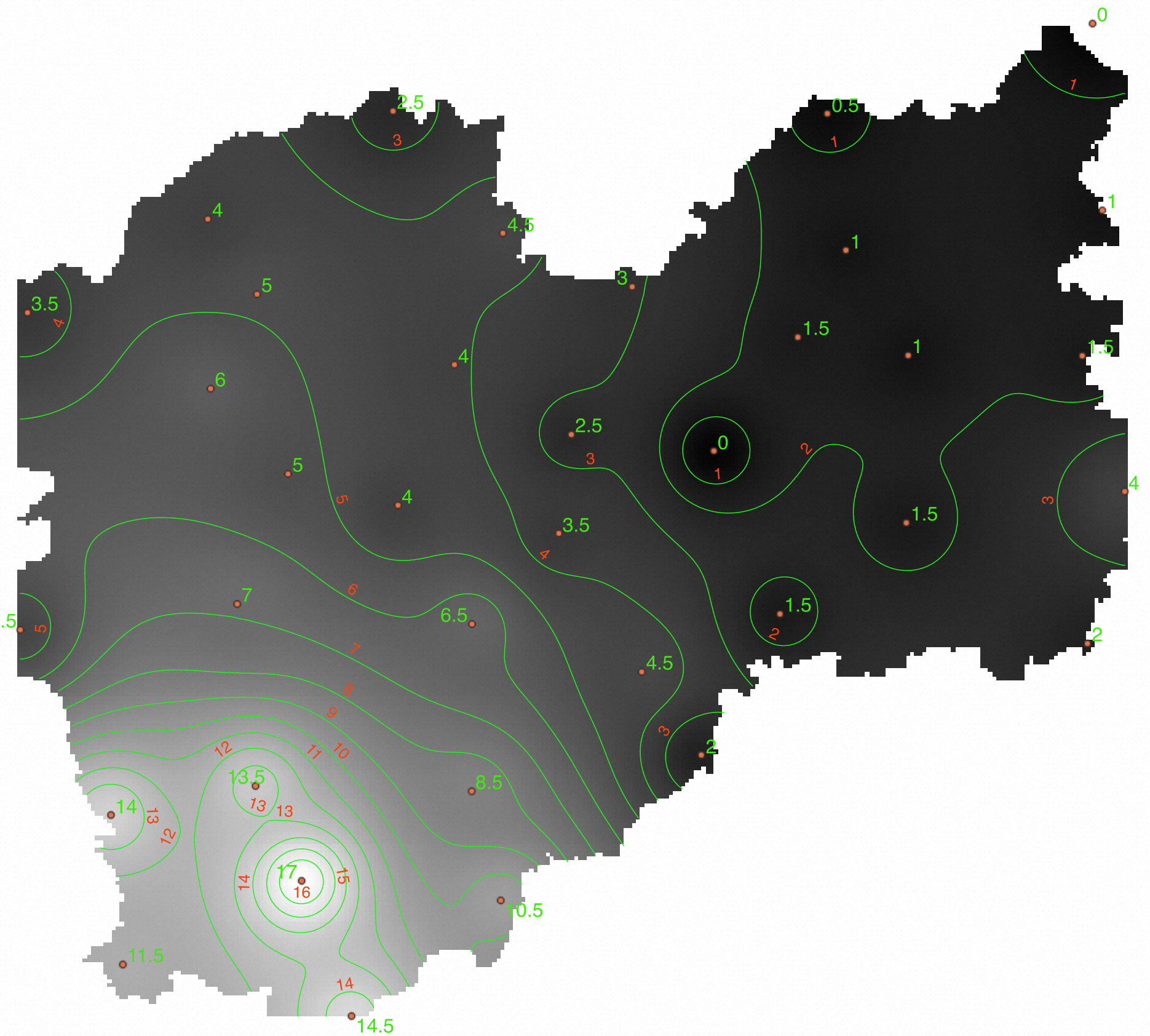
Contour lines connect grid cells with equal precipitation values. In hydrology, these are called isohyets. An interval of 1.0 means each contour line represents a 1 mm difference in precipitation. Generating contours helps visualize the spatial distribution of precipitation across the study area.
Generate contour lines
traces contours from the raster and intersects them with the administrative boundary polygon:
CREATE TABLE rs_contours AS
SELECT id, max_value, min_value, ST_Intersection(a.geom, p.geom)
FROM (
  SELECT (ST_Contour(rast, 1, '{"interval":"1.0"}')).*
  FROM raster_table WHERE id = 1
) a, polygon_table AS p;
Import rs_contours into QGIS for visualization. In the following image, green numbers are precipitation values at observation sites; red numbers are contour values:
Generate surfaces
To generate polygon surfaces instead of lines, set "polygonize":"true" in the options:
CREATE TABLE rs_contours_polygon AS
SELECT id, max_value, min_value, ST_Intersection(a.geom, p.geom)
FROM (
  SELECT (ST_Contour(rast, 1, '{"interval":"1.0","polygonize":"true"}')).*
  FROM raster_table WHERE id = 1
) a, polygon_table AS p;
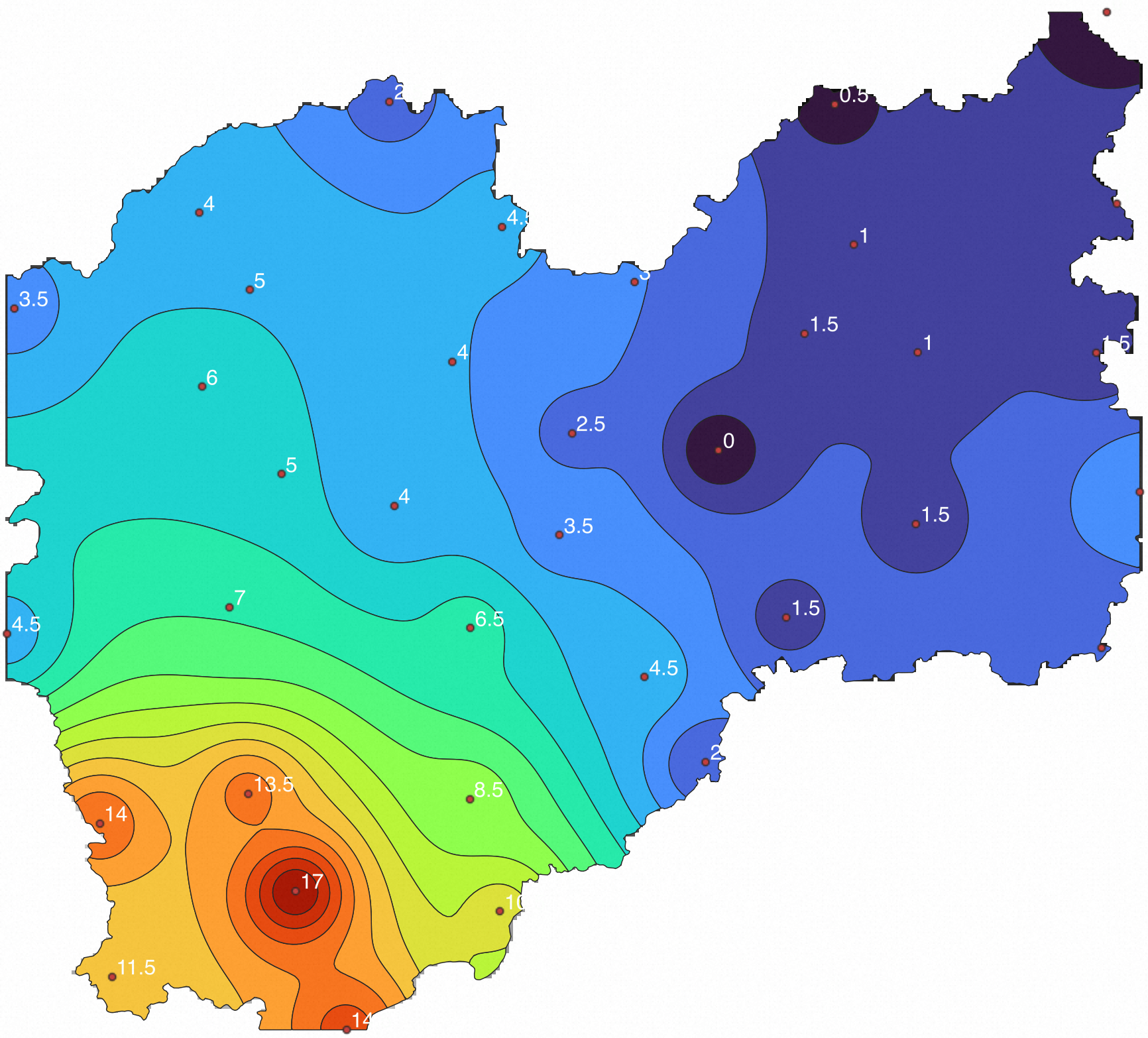
Each surface polygon covers the area between two consecutive contour values. The following QGIS image shows the colored surfaces overlaid on the boundary:
Calculate areal precipitation
Areal precipitation is the ratio of total precipitation over an area to the size of that area, expressed in mm/m². The calculation weights each pixel's precipitation value by the area it covers, sums these weighted values, and divides by the total pixel area:
areal precipitation = sum(pixel_area × precipitation) / sum(pixel_area)Step 1: Collect interval statistics.
returns statistics on pixel values within any polygon area. This example uses the interval (0,5,10,15,20] to break down the precipitation distribution:
SELECT (ST_Statistics(
  rast,
  ST_GeomFromText('POLYGON((119.0969 28.0519, 118.9058 27.8942, 119.0502 27.5649,
    119.3347 27.6292, 119.4262 27.8775, 119.4927 28.1823,
    119.3812 28.1186, 119.0969 28.0519))'),
  0,
  '(0,5,10,15,20]',
  false
)).*
FROM raster_table
WHERE id = 1;
Expected output:
  name    | band |   min   |   max   |  mean   |    sum     | count |  std  | median |  mode
----------+------+---------+---------+---------+------------+-------+-------+--------+-------
 full     |    0 |  2.5010 | 16.8416 |  6.6184 | 243748.59  | 36829 | 2.686 |  6.046 | 3.892
 (0-5]    |    0 |  2.5010 |  4.9999 |  4.1440 |  50963.11  | 12298 | 0.553 |  4.232 | 3.892
 (5-10]   |    0 |  5.0000 |  9.9999 |  6.8528 | 136110.09  | 19862 | 1.293 |  6.623 | 5.028
 (10-15]  |    0 | 10.0001 | 14.9939 | 11.9475 |  52999.25  |  4436 | 1.228 | 11.901 | 12.431
 (15-20]  |    0 | 15.0045 | 16.8416 | 15.7774 |   3676.14  |   233 | 0.509 | 15.735 | 15.004
(5 rows)
Output columns:
| Column | Description |
|---|---|
name |
Interval label — full covers all pixels; (0-5] covers pixels with values greater than 0 and up to 5 |
band |
Band index (0-based) |
min / max |
Minimum and maximum pixel values in the interval |
mean |
Average pixel value |
sum |
Sum of all pixel values in the interval |
count |
Number of pixels in the interval |
std |
Standard deviation |
median |
Median pixel value |
mode |
Most frequently occurring pixel value |
From this output: the maximum precipitation in the polygon is 16.84 mm, the minimum is 2.50 mm, and 4,436 pixels have values between 10 mm and 15 mm.
Step 2: Clip the raster to the target polygon.
INSERT INTO raster_table
SELECT 3, ST_ClipToRast(
  rast,
  ST_GeomFromText('POLYGON((119.0969 28.0519, 118.9058 27.8942, 119.0502 27.5649,
    119.3347 27.6292, 119.4262 27.8775, 119.4927 28.1823,
    119.3812 28.1186, 119.0969 28.0519))'),
  0, '', NULL, '', '{"chunktable":"rbt"}'
)
FROM raster_table WHERE id = 1;
Check the dimensions of the clipped raster:
SELECT ST_Width(rast), ST_Height(rast) FROM raster_table WHERE id = 3;Expected output:
 st_width | st_height
----------+-----------
      185 |       217
(1 row)
Step 3: Extract the area and precipitation value for each pixel.
returns the rectangular polygon covered by each pixel; ST_Value returns the pixel's precipitation value. Traverse all 185 × 217 pixels and store the results:
-- Create a table to store per-pixel data
CREATE TABLE pixel_pre (
  row  integer,
  col  integer,
  geom geometry,        -- polygon covered by the pixel
  pre  double precision -- precipitation value of the pixel
);

-- Set the spatial reference
UPDATE raster_table SET rast = ST_SetSrid(rast, 4326);

-- Traverse each pixel and collect its covered area and value
DO
$do$
BEGIN
  FOR i IN 0..184 LOOP
    FOR j IN 0..216 LOOP
      INSERT INTO pixel_pre
      SELECT i, j,
             ST_PixelAsPolygon(rast, j, i),
             ST_Value(rast, 0, i, j) AS value
      FROM raster_table
      WHERE id = 3;
    END LOOP;
  END LOOP;
END
$do$;
Verify the result:
SELECT row, col, ST_AsText(geom), pre FROM pixel_pre LIMIT 10;Expected output (each row shows a pixel's coordinates, covered rectangular area, and precipitation value):
 row | col |                        st_astext                        |        pre
-----+-----+----------------------------------------------------------+--------------------
 107 |  33 | POLYGON((119.2448 28.0907,...,119.2448 28.0907))         |   5.666
 107 |  34 | POLYGON((119.2448 28.0879,...,119.2448 28.0879))         |   5.699
 ...
(10 rows)
Step 4: Compute the weighted areal precipitation.
Convert coordinates from EPSG:4326 to EPSG:3857 to get pixel areas in square meters. Then apply the weighted average formula:
SELECT sum(ST_Area(ST_Transform(geom, 3857)) * pre)
       / sum(ST_Area(ST_Transform(geom, 3857))) AS "precipitation (mm/m²)"
FROM pixel_pre
WHERE pre > 0;
Expected output:
 precipitation (mm/m²)
-----------------------
     9.434021577002174
(1 row)
The areal precipitation for this polygon is approximately 9.43 mm/m².
Conclusion
GanosBase Raster provides a complete in-database toolkit for raster data import, storage, analysis, and visualization. It meets the requirements of remote sensing image management, DEM data analysis, and grid data analysis, and offers advanced capabilities such as GPU computation to support various applications. GanosBase Raster supports use cases across meteorology, water conservancy, resource management, emergency response, and more. In the Ministry of Water Resources' meteorological precipitation consultation system, GanosBase Raster improved analysis and calculation efficiency by more than 10 times compared to the previous approach. With comprehensive capabilities and application cases in water resources, natural resources, meteorology, environmental protection, and emergency response, GanosBase Raster provides robust spatio-temporal foundational support for aerospace big data management applications.