Choosing the right Hologres table properties for your query patterns reduces the amount of data scanned, the number of files accessed, and the number of I/O operations — resulting in lower latency and higher queries per second (QPS). This guide maps six common query scenarios to the storage format, primary key, distribution key, clustering key, partitioning, and bitmap index settings that best fit each one.
Choose a storage format
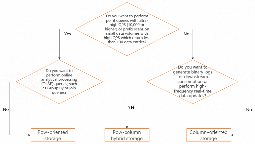
Hologres supports three storage formats: row-oriented storage, column-oriented storage, and row-column hybrid storage. For details on each format, see Set up data orientation.
Use the following decision tree to select a format. If your workload is not yet well-defined, start with row-column hybrid storage — it balances trade-offs across the widest range of query patterns.
Property quick reference
Each table property targets a specific layer of query execution. Understanding what each one does helps you choose the right combination for your scenario.
| Property | What it does | Best for |
|---|---|---|
| Primary key | Enables Fixed Plan for direct row lookup | Point queries with ultra-high QPS |
| Distribution key | Co-locates rows on the same shard by key value; reduces cross-shard shuffle | Aggregate queries; JOIN queries |
| Clustering key | Physically sorts rows by key within each file; reduces I/O for range or equality scans | Prefix scans; single-value filter queries |
event_time_column (segment key) |
Sorts data within each file by this column; reduces files scanned for range predicates | Time-based filter queries |
| Partitioning | Prunes entire partitions before scanning | Large tables with time-based access patterns |
| Bitmap index | Maps each distinct value to matching rows; narrows scans for single-value filters | Single-value filter queries |
Configure table properties by query scenario
Once you have a storage format, align the remaining table properties with your query patterns. Each scenario below describes the recommended configuration, explains the mechanism, and shows measured performance results.
The examples in this section use a 64 compute unit (CU) Hologres instance and the TPC-H 100 GB dataset. The dataset contains two tables: the Orders table (whereo_orderkeyuniquely identifies an order) and the Lineitem table (wherel_orderkeyandl_linenumbertogether identify a line item). These tests are based on the TPC-H benchmarking methodology but do not meet all TPC-H requirements; results cannot be compared with published TPC-H benchmark results. If your table serves multiple query patterns with different filter or JOIN fields, configure properties based on your most frequent or most performance-sensitive query.
Scenario 1: Point queries with ultra-high QPS
Query pattern
You want to perform tens of thousands of point queries per second on the Orders table. You can specify the o_orderkey field to locate a row of data.
SELECT * FROM orders WHERE o_orderkey = ?;Configuration
Set the filter field as the primary key. Hologres generates a Fixed Plan for primary-key lookups, bypassing the general query planning path and significantly reducing execution overhead. For details, see Accelerate SQL execution with Fixed Plan.
How it works
The Fixed Plan skips query optimization steps that are unnecessary for single-row lookups, routing requests directly to the target row. Without a primary key, the engine falls back to a full shard scan.
Performance results (500 concurrent queries, row-oriented or row-column hybrid table)
| Configuration | Avg QPS | Avg latency |
|---|---|---|
| Primary key configured | ~104,000 | ~4 ms |
| No primary key | ~16,000 | ~30 ms |
For the DDL statement, see Scenario 1 DDL.
Scenario 2: Prefix scans on a small dataset with high QPS
Query pattern
You want to perform queries with the following characteristics: tens of thousands of QPS need to be processed, queries are performed based on a field in the primary key, and the returned dataset contains several or dozens of data entries.
SELECT * FROM lineitem WHERE l_orderkey = ?;This query retrieves all line items for one order — a prefix scan on a composite primary key.
Configuration
Apply all three of the following:
-
Primary key ordering — Put the filter field first in the composite primary key. Use
(l_orderkey, l_linenumber), not(l_linenumber, l_orderkey). This lets Hologres evaluate the equality predicate against the leading key without scanning unrelated rows. -
Distribution key — Set the filter field as the distribution key (
l_orderkey). Data for each order is stored within a single shard, so the query touches exactly one shard instead of all shards. -
Clustering key (column-oriented or row-column hybrid storage only) — Set the filter field as the clustering key (
l_orderkey). Within each file, rows are sorted by this key, reducing I/O when scanning a contiguous range.
With these properties in place, enable the Fixed Plan for prefix scans by setting the Grand Unified Configuration (GUC) parameter hg_experimental_enable_fixed_dispatcher_for_scan to on. For details, see Accelerate SQL execution with Fixed Plan.
How it works
The combination of correct primary key ordering, a co-located distribution key, and a clustering key means that all matching rows are in one shard, physically adjacent in storage, and directly addressed by the Fixed Plan.
Performance results (row-oriented or row-column hybrid table)
| Configuration | Concurrent queries | Avg QPS | Avg latency |
|---|---|---|---|
| All three properties configured | 500 | ~37,000 | ~13 ms |
| Properties not configured | 1 | ~60 | ~16 ms |
For the DDL statement, see Scenario 2 DDL.
Scenario 3: Queries with time-based filter conditions
Query pattern
-- Original query
SELECT
    l_returnflag,
    l_linestatus,
    sum(l_quantity) AS sum_qty,
    sum(l_extendedprice) AS sum_base_price,
    sum(l_extendedprice * (1 - l_discount)) AS sum_disc_price,
    sum(l_extendedprice * (1 - l_discount) * (1 + l_tax)) AS sum_charge,
    avg(l_quantity) AS avg_qty,
    avg(l_extendedprice) AS avg_price,
    avg(l_discount) AS avg_disc,
    count(*) AS count_order
FROM
    lineitem
WHERE
    l_shipdate <= date '1998-12-01' - interval '120' day
GROUP BY
    l_returnflag,
    l_linestatus
ORDER BY
    l_returnflag,
    l_linestatus;

-- Modified query used in the performance test (narrowed time range to highlight the effect)
SELECT ... FROM lineitem
WHERE
    l_year='1992'               -- filters to a single partition
    AND l_shipdate <= date '1992-12-01'
...;
Configuration
-
Partition by time — Add an
l_yearcolumn and use it as the partition key to split the table by year. Determine whether to partition your table or only configure theevent_time_columnproperty based on your data volume and business requirements. Check the limits and usage notes in CREATE PARTITION TABLE before partitioning. -
`event_time_column` — Set
l_shipdateas theevent_time_column(segment key). This ensures that data entries in files in the shard are sorted in order based on theevent_time_columnproperty, which reduces the number of files to be scanned. For details, see Event Time Column (Segment Key).
How it works
Partitioning prunes entire partitions before the query reads any file. The event_time_column then prunes individual files within the remaining partition by sorting data within each file by the configured column.
Performance results (column-oriented table)
| Configuration | Files scanned |
|---|---|
Partition + event_time_column configured as suggested |
80 files in 1 partition |
No partition; event_time_column set to a different field |
320 files |
RunEXPLAIN ANALYZEto inspect actual scan counts. ThePartitions selectedparameter shows how many partitions were accessed; thedopparameter shows how many files were scanned.
For the DDL statement, see Scenario 3 DDL.
Scenario 4: Queries with non-time single-value filter conditions
Query pattern
SELECT
    ...
FROM
    lineitem
WHERE
    l_shipmode IN ('FOB', 'AIR');
Configuration
-
Clustering key — Set
l_shipmodeas the clustering key. Rows with the samel_shipmodevalue are stored consecutively in each file, so the engine reads a smaller, contiguous block instead of scattered rows across the file. -
Bitmap index — Configure
l_shipmodeas a bitmap column. The bitmap index maps each distinct value to the rows that contain it, letting the engine jump directly to matching rows without reading unrelated data.
How it works
The clustering key reduces I/O by grouping matching rows physically. The bitmap index then narrows the scan further by filtering at the block level before any row data is read.
Performance results (column-oriented table)
| Configuration | Rows read | Query duration |
|---|---|---|
| Clustering key + bitmap index configured | 170 million | 0.71 s |
| Neither configured | 600 million (full table) | 2.41 s |
Check the number of rows read via theread_rowsparameter in slow query logs. See Get and analyze slow query logs. To confirm that the bitmap index is being applied, look for theBitmap Filterkeyword in the execution plan.
For the DDL statement, see Scenario 4 DDL.
Scenario 5: Aggregate queries on a single field
Query pattern
SELECT
    l_suppkey,
    sum(l_extendedprice * (1 - l_discount))
FROM
    lineitem
GROUP BY
    l_suppkey;
Configuration
Set the GROUP BY field (l_suppkey) as the distribution key. When data is already distributed by the aggregation key, each shard computes its local aggregate independently — no data needs to move between shards.
How it works
Without a matching distribution key, the engine shuffles all rows to a set of reducer shards before aggregating. With a matching distribution key, this prevents a large amount of data from being shuffled across shards.
Performance results (column-oriented table)
| Configuration | Data shuffled | Execution duration |
|---|---|---|
l_suppkey as distribution key |
~0.21 GB | 2.30 s |
| Different field as distribution key | ~8.16 GB | 3.68 s |
Check the volume of shuffled data via the shuffle_bytes parameter in slow query logs. See Get and analyze slow query logs.
For the DDL statement, see Scenario 5 DDL.
Scenario 6: JOIN queries across multiple tables
Query pattern
SELECT
    o_orderpriority,
    count(*) AS order_count
FROM
    orders
WHERE
    o_orderdate >= date '1996-07-01'
    AND o_orderdate < date '1996-07-01' + interval '3' month
    AND EXISTS (
        SELECT
            *
        FROM
            lineitem
        WHERE
            l_orderkey = o_orderkey    -- join condition
            AND l_commitdate < l_receiptdate)
GROUP BY
    o_orderpriority
ORDER BY
    o_orderpriority;
Configuration
Set the JOIN fields as distribution keys on both tables:
-
Lineitem:
l_orderkeyas the distribution key -
Orders:
o_orderkeyas the distribution key
When both tables are distributed on the same key, matching rows from each table are already co-located on the same shard. The JOIN executes locally without shuffling either table across the network.
How it works
When tables are distributed on different keys, a large amount of data must be shuffled across shards to execute the JOIN. Aligning distribution keys with JOIN fields prevents this large-scale data shuffle and turns a network-bound operation into a local one.
Performance results (both tables column-oriented)
| Configuration | Data shuffled | Execution duration |
|---|---|---|
| JOIN fields as distribution keys on both tables | ~0.45 GB | 2.19 s |
| Distribution keys not aligned with JOIN fields | ~6.31 GB | 5.55 s |
Check the volume of shuffled data via the shuffle_bytes parameter in slow query logs. See Get and analyze slow query logs.
For the DDL statements, see Scenario 6 DDL.
(Optional) Assign tables to table groups
If your Hologres instance has more than 256 cores and serves a variety of workloads, configure multiple table groups and assign each table to the appropriate group at creation time. This isolates resource usage across workloads. For details, see Best practices for table group setup.
Appendix: DDL statements
Scenario 1 DDL
-- Create the Orders table with a primary key.
-- To create the table without a primary key, remove PRIMARY KEY from the O_ORDERKEY column.
DROP TABLE IF EXISTS orders;
BEGIN;
CREATE TABLE orders(
    O_ORDERKEY       BIGINT         NOT NULL PRIMARY KEY
    ,O_CUSTKEY       INT            NOT NULL
    ,O_ORDERSTATUS   TEXT           NOT NULL
    ,O_TOTALPRICE    DECIMAL(15,2)  NOT NULL
    ,O_ORDERDATE     TIMESTAMPTZ    NOT NULL
    ,O_ORDERPRIORITY TEXT           NOT NULL
    ,O_CLERK         TEXT           NOT NULL
    ,O_SHIPPRIORITY  INT            NOT NULL
    ,O_COMMENT       TEXT           NOT NULL
);
CALL SET_TABLE_PROPERTY('orders', 'orientation', 'row');
CALL SET_TABLE_PROPERTY('orders', 'clustering_key', 'o_orderkey');
CALL SET_TABLE_PROPERTY('orders', 'distribution_key', 'o_orderkey');
COMMIT;
Scenario 2 DDL
-- Create the Lineitem table with properties configured for prefix scan optimization.
DROP TABLE IF EXISTS lineitem;
BEGIN;
CREATE TABLE lineitem
(
    L_ORDERKEY      BIGINT      NOT NULL,
    L_PARTKEY       INT         NOT NULL,
    L_SUPPKEY       INT         NOT NULL,
    L_LINENUMBER    INT         NOT NULL,
    L_QUANTITY      DECIMAL(15,2) NOT NULL,
    L_EXTENDEDPRICE DECIMAL(15,2) NOT NULL,
    L_DISCOUNT      DECIMAL(15,2) NOT NULL,
    L_TAX           DECIMAL(15,2) NOT NULL,
    L_RETURNFLAG    TEXT        NOT NULL,
    L_LINESTATUS    TEXT        NOT NULL,
    L_SHIPDATE      TIMESTAMPTZ NOT NULL,
    L_COMMITDATE    TIMESTAMPTZ NOT NULL,
    L_RECEIPTDATE   TIMESTAMPTZ NOT NULL,
    L_SHIPINSTRUCT  TEXT        NOT NULL,
    L_SHIPMODE      TEXT        NOT NULL,
    L_COMMENT       TEXT        NOT NULL,
    PRIMARY KEY (L_ORDERKEY,L_LINENUMBER)
);
CALL set_table_property('lineitem', 'orientation', 'row');
-- CALL set_table_property('lineitem', 'clustering_key', 'L_ORDERKEY,L_SHIPDATE');
CALL set_table_property('lineitem', 'distribution_key', 'L_ORDERKEY');
COMMIT;
Scenario 3 DDL
-- Create a partitioned Lineitem table partitioned by year.
-- The non-partitioned version uses the same DDL as Scenario 2.
DROP TABLE IF EXISTS lineitem;
BEGIN;
CREATE TABLE lineitem
(
    L_ORDERKEY      BIGINT      NOT NULL,
    L_PARTKEY       INT         NOT NULL,
    L_SUPPKEY       INT         NOT NULL,
    L_LINENUMBER    INT         NOT NULL,
    L_QUANTITY      DECIMAL(15,2) NOT NULL,
    L_EXTENDEDPRICE DECIMAL(15,2) NOT NULL,
    L_DISCOUNT      DECIMAL(15,2) NOT NULL,
    L_TAX           DECIMAL(15,2) NOT NULL,
    L_RETURNFLAG    TEXT        NOT NULL,
    L_LINESTATUS    TEXT        NOT NULL,
    L_SHIPDATE      TIMESTAMPTZ NOT NULL,
    L_COMMITDATE    TIMESTAMPTZ NOT NULL,
    L_RECEIPTDATE   TIMESTAMPTZ NOT NULL,
    L_SHIPINSTRUCT  TEXT        NOT NULL,
    L_SHIPMODE      TEXT        NOT NULL,
    L_COMMENT       TEXT        NOT NULL,
    L_YEAR          TEXT        NOT NULL,
    PRIMARY KEY (L_ORDERKEY,L_LINENUMBER,L_YEAR)
)
PARTITION BY LIST (L_YEAR);
CALL set_table_property('lineitem', 'clustering_key', 'L_ORDERKEY,L_SHIPDATE');
CALL set_table_property('lineitem', 'segment_key', 'L_SHIPDATE');
CALL set_table_property('lineitem', 'distribution_key', 'L_ORDERKEY');
COMMIT;
Scenario 4 DDL
-- Create the Lineitem table without clustering key or bitmap index (baseline).
-- For the optimized version, add the clustering key and bitmap_columns properties as shown in the comments.
DROP TABLE IF EXISTS lineitem;
BEGIN;
CREATE TABLE lineitem
(
    L_ORDERKEY      BIGINT      NOT NULL,
    L_PARTKEY       INT         NOT NULL,
    L_SUPPKEY       INT         NOT NULL,
    L_LINENUMBER    INT         NOT NULL,
    L_QUANTITY      DECIMAL(15,2) NOT NULL,
    L_EXTENDEDPRICE DECIMAL(15,2) NOT NULL,
    L_DISCOUNT      DECIMAL(15,2) NOT NULL,
    L_TAX           DECIMAL(15,2) NOT NULL,
    L_RETURNFLAG    TEXT        NOT NULL,
    L_LINESTATUS    TEXT        NOT NULL,
    L_SHIPDATE      TIMESTAMPTZ NOT NULL,
    L_COMMITDATE    TIMESTAMPTZ NOT NULL,
    L_RECEIPTDATE   TIMESTAMPTZ NOT NULL,
    L_SHIPINSTRUCT  TEXT        NOT NULL,
    L_SHIPMODE      TEXT        NOT NULL,
    L_COMMENT       TEXT        NOT NULL,
    PRIMARY KEY (L_ORDERKEY,L_LINENUMBER)
);
CALL set_table_property('lineitem', 'segment_key', 'L_SHIPDATE');
CALL set_table_property('lineitem', 'distribution_key', 'L_ORDERKEY');
CALL set_table_property('lineitem', 'bitmap_columns', 'l_orderkey,l_partkey,l_suppkey,l_linenumber,l_returnflag,l_linestatus,l_shipinstruct,l_comment');
COMMIT;
Scenario 5 DDL
-- Create the Lineitem table with the GROUP BY field configured as the distribution key.
DROP TABLE IF EXISTS lineitem;
BEGIN;
CREATE TABLE lineitem
(
    L_ORDERKEY      BIGINT      NOT NULL,
    L_PARTKEY       INT         NOT NULL,
    L_SUPPKEY       INT         NOT NULL,
    L_LINENUMBER    INT         NOT NULL,
    L_QUANTITY      DECIMAL(15,2) NOT NULL,
    L_EXTENDEDPRICE DECIMAL(15,2) NOT NULL,
    L_DISCOUNT      DECIMAL(15,2) NOT NULL,
    L_TAX           DECIMAL(15,2) NOT NULL,
    L_RETURNFLAG    TEXT        NOT NULL,
    L_LINESTATUS    TEXT        NOT NULL,
    L_SHIPDATE      TIMESTAMPTZ NOT NULL,
    L_COMMITDATE    TIMESTAMPTZ NOT NULL,
    L_RECEIPTDATE   TIMESTAMPTZ NOT NULL,
    L_SHIPINSTRUCT  TEXT        NOT NULL,
    L_SHIPMODE      TEXT        NOT NULL,
    L_COMMENT       TEXT        NOT NULL,
    PRIMARY KEY (L_ORDERKEY,L_LINENUMBER,L_SUPPKEY)
);
CALL set_table_property('lineitem', 'segment_key', 'L_COMMITDATE');
CALL set_table_property('lineitem', 'clustering_key', 'L_ORDERKEY,L_SHIPDATE');
CALL set_table_property('lineitem', 'distribution_key', 'L_SUPPKEY');
COMMIT;
Scenario 6 DDL
DROP TABLE IF EXISTS LINEITEM;

BEGIN;
CREATE TABLE LINEITEM
(
    L_ORDERKEY      BIGINT      NOT NULL,
    L_PARTKEY       INT         NOT NULL,
    L_SUPPKEY       INT         NOT NULL,
    L_LINENUMBER    INT         NOT NULL,
    L_QUANTITY      DECIMAL(15,2) NOT NULL,
    L_EXTENDEDPRICE DECIMAL(15,2) NOT NULL,
    L_DISCOUNT      DECIMAL(15,2) NOT NULL,
    L_TAX           DECIMAL(15,2) NOT NULL,
    L_RETURNFLAG    TEXT        NOT NULL,
    L_LINESTATUS    TEXT        NOT NULL,
    L_SHIPDATE      TIMESTAMPTZ NOT NULL,
    L_COMMITDATE    TIMESTAMPTZ NOT NULL,
    L_RECEIPTDATE   TIMESTAMPTZ NOT NULL,
    L_SHIPINSTRUCT  TEXT        NOT NULL,
    L_SHIPMODE      TEXT        NOT NULL,
    L_COMMENT       TEXT        NOT NULL,
    PRIMARY KEY (L_ORDERKEY,L_LINENUMBER)
);
CALL set_table_property('LINEITEM', 'clustering_key', 'L_SHIPDATE,L_ORDERKEY');
CALL set_table_property('LINEITEM', 'segment_key', 'L_SHIPDATE');
CALL set_table_property('LINEITEM', 'distribution_key', 'L_ORDERKEY');
CALL set_table_property('LINEITEM', 'bitmap_columns', 'L_ORDERKEY,L_PARTKEY,L_SUPPKEY,L_LINENUMBER,L_RETURNFLAG,L_LINESTATUS,L_SHIPINSTRUCT,L_SHIPMODE,L_COMMENT');
CALL set_table_property('LINEITEM', 'dictionary_encoding_columns', 'L_RETURNFLAG,L_LINESTATUS,L_SHIPINSTRUCT,L_SHIPMODE,L_COMMENT');
COMMIT;

DROP TABLE IF EXISTS ORDERS;

BEGIN;
CREATE TABLE ORDERS
(
    O_ORDERKEY      BIGINT      NOT NULL PRIMARY KEY,
    O_CUSTKEY       INT         NOT NULL,
    O_ORDERSTATUS   TEXT        NOT NULL,
    O_TOTALPRICE    DECIMAL(15,2) NOT NULL,
    O_ORDERDATE     timestamptz NOT NULL,
    O_ORDERPRIORITY TEXT        NOT NULL,
    O_CLERK         TEXT        NOT NULL,
    O_SHIPPRIORITY  INT         NOT NULL,
    O_COMMENT       TEXT        NOT NULL
);
CALL set_table_property('ORDERS', 'segment_key', 'O_ORDERDATE');
CALL set_table_property('ORDERS', 'distribution_key', 'O_ORDERKEY');
CALL set_table_property('ORDERS', 'bitmap_columns', 'O_ORDERKEY,O_CUSTKEY,O_ORDERSTATUS,O_ORDERPRIORITY,O_CLERK,O_SHIPPRIORITY,O_COMMENT');
CALL set_table_property('ORDERS', 'dictionary_encoding_columns', 'O_ORDERSTATUS,O_ORDERPRIORITY,O_CLERK,O_COMMENT');
COMMIT;
References
For Data Definition Language (DDL) statements for Hologres internal tables, see: