After you migrate data from a self-managed ClickHouse cluster to the cloud, you may encounter compatibility and performance issues. To ensure a smooth migration, we recommend running this analysis in a test environment before switching production traffic.
Background information
Self-managed ClickHouse clusters migrated to ApsaraDB for ClickHouse may encounter the following issues:
-
Version compatibility issues:
-
MaterializedMySQL engine compatibility issues
-
SQL compatibility issues
-
-
CPU resources exhausted and memory insufficient after migrating to ApsaraDB for ClickHouse
To resolve these issues, focus on compatibility and performance during the migration.
This guide covers:
-
Parameter compatibility — compare settings between clusters and align them
-
MaterializedMySQL compatibility — handle engine differences after migration
-
SQL compatibility verification — batch-test your existing queries against the new cluster
-
Performance bottleneck analysis — locate the tables and queries causing CPU or memory issues
-
SQL optimization — apply targeted fixes after identifying the root cause
Compatibility analysis
Parameter compatibility
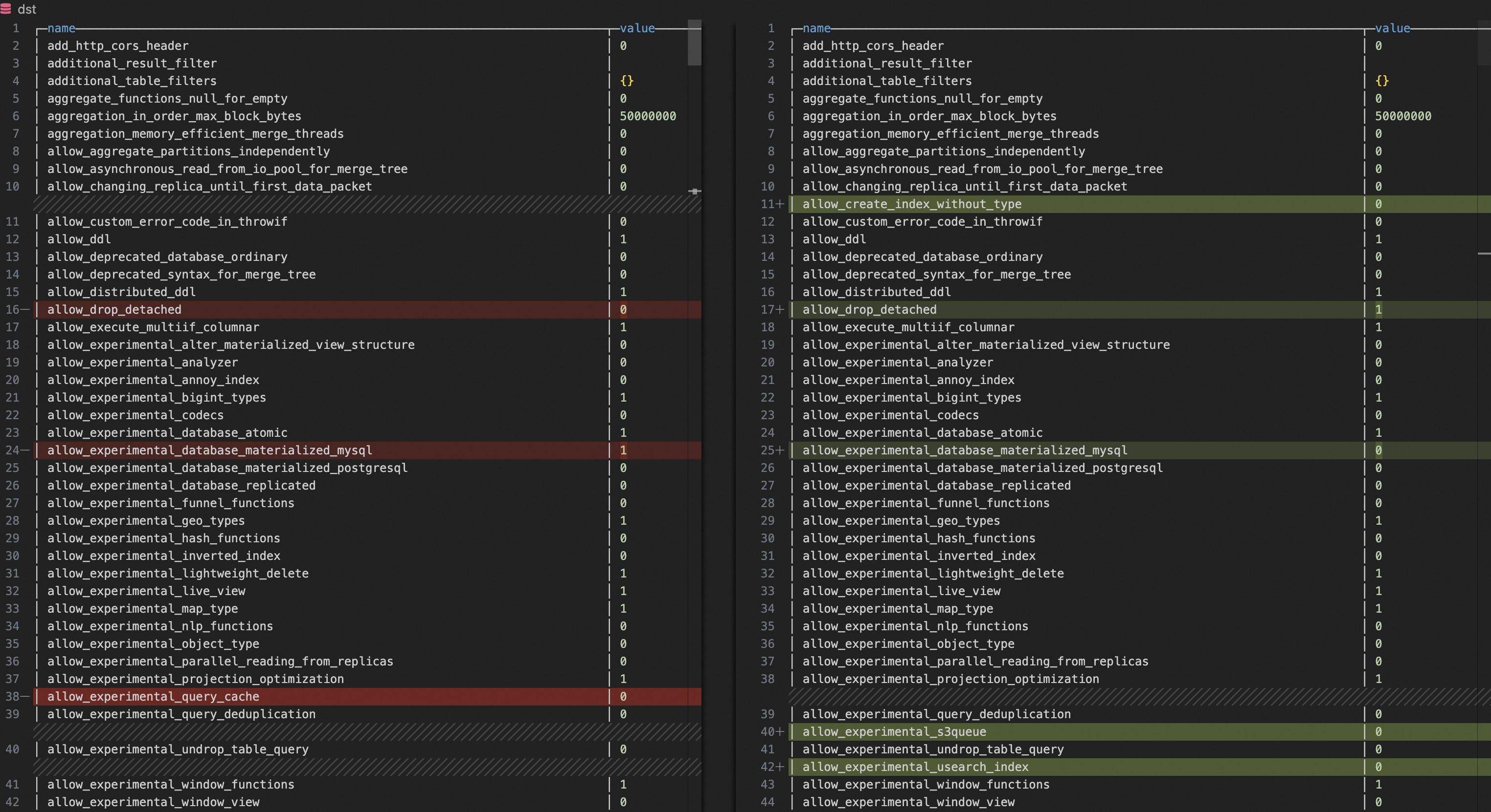
Run this query on both your self-managed cluster and your ApsaraDB for ClickHouse cluster to export all configuration parameters:
SELECT
    name,
    groupArrayDistinct(value) AS value
FROM clusterAllReplicas(`default`, system.settings)
GROUP BY name
ORDER BY name ASC
Then use a diff tool (such as VS Code's built-in file comparison) to identify mismatches. For any parameter that differs, update the ApsaraDB for ClickHouse cluster to match the self-managed cluster's value.
Parameters that affect compatibility:
-
compatibility -
prefer_global_in_and_join -
distributed_product_mode
Parameters that affect performance:
-
max_threads -
max_bytes_to_merge_at_max_space_in_pool -
prefer_global_in_and_join
MaterializedMySQL compatibility
If your self-managed cluster synchronizes data from MySQL using the MaterializedMySQL engine, be aware of how ApsaraDB for ClickHouse handles this after migration.
The community version of the MaterializedMySQL engine is no longer maintained. ApsaraDB for ClickHouse uses Data Transmission Service (DTS) to sync MySQL data instead. DTS creates a ReplacingMergeTree local table on each cluster node and a distributed table that routes writes to those nodes — replacing the MaterializedMySQL table entirely.
This architectural change causes two common issues:
Issue 1: IN and JOIN queries break on the distributed table
In the self-managed cluster, MaterializedMySQL replicates data to each shard directly. After migration, data flows through a distributed table, which changes how IN and JOIN subqueries resolve. For details and fixes, see What do I do if an error occurs when I use a subquery on a distributed table?.
Issue 2: Duplicate data in query results
The ReplacingMergeTree table merges duplicate rows asynchronously in the background. If merges fall behind, queries return more duplicates than the self-managed cluster did. Two solutions are available:
Solution 1: Force deduplication at query time
Run the following command to enable the final modifier globally. This deduplicates results during each query but increases CPU and memory usage:
SET global final = 1;Solution 2: Tune merge frequency on the target table
Increase how often ApsaraDB for ClickHouse merges parts in the ReplacingMergeTree table:
ALTER TABLE <AIM_TABLE>
    MODIFY SETTING
        min_age_to_force_merge_on_partition_only = 1,
min_age_to_force_merge_seconds = 60;| Parameter | Description | Default |
|---|---|---|
min_age_to_force_merge_on_partition_only |
When set to 1, forces data merging within partitions |
0 (disabled) |
min_age_to_force_merge_seconds |
Time interval between forced part merges (in seconds) | 3600 |
SQL compatibility verification
Use a Python script to extract SELECT statements from your self-managed cluster's query log and replay them against ApsaraDB for ClickHouse. Failed queries indicate SQL compatibility issues to resolve before migration.
Prerequisites
Before you begin, ensure that you have:
-
A Python 3 environment on the verification server. An Alibaba Cloud Elastic Compute Service (ECS) instance running Linux already includes Python 3. If you're not using ECS, install Python 3 from the Python official website.
-
Network connectivity from the verification server to both clusters. For connectivity troubleshooting, see How do I resolve network connectivity issues between the target cluster and the data source?
Verify SQL compatibility
-
Install the Python client library for ClickHouse:
pip3 install clickhouse_driver -
Create a Python file with the following script. Replace the placeholder values with your actual connection details:
from clickhouse_driver import connect import datetime import logging # pip3 install clickhouse_driver is required. # Connection settings for the self-managed cluster host_old = 'HOST_OLD' # VPC endpoint port_old = TCP_PORT_OLD # TCP port user_old = 'USER_OLD' # Username password_old = 'PASSWORD_OLD' # Password # Connection settings for ApsaraDB for ClickHouse host_new = 'HOST_NEW' # VPC endpoint port_new = TCP_PORT_NEW # TCP port user_new = 'USER_NEW' # Username password_new = 'PASSWORD_NEW' # Password logging.basicConfig(level=logging.INFO, format='%(asctime)s - %(levelname)s - %(message)s') def create_connection(host, port, user, password): """Establish a connection to ClickHouse.""" return connect(host=host, port=port, user=user, password=password) def get_query_hashes(cursor): """Query the query_hash list of the last two days.""" get_queryhash_sql = ''' select distinct normalized_query_hash from system.query_log where type='QueryFinish' and `is_initial_query`=1 and `user` not in ('default', 'aurora') and lower(`query`) not like 'select 1%' and lower(`query`) not like 'select timezone()%' and lower(`query`) not like '%dms-websql%' and lower(`query`) like 'select%' and `event_time` > now() - INTERVAL 2 DAY; ''' cursor.execute(get_queryhash_sql) return cursor.fetchall() def get_sql_info(cursor, queryhash): """Query the SQL information for the specified query_hash in the last 2 days (search range is 3 days).""" get_sqlinfo_sql = f''' select `event_time`, `query_duration_ms`, `read_rows`, `read_bytes`, `memory_usage`, `databases`, `tables`, `current_database`, `query` from system.query_log where `event_time` > now() - INTERVAL 3 DAY and `type`='QueryFinish' and `normalized_query_hash`='{queryhash}' limit 1 ''' cursor.execute(get_sqlinfo_sql) sql_info = cursor.fetchone() if sql_info: return [info.strftime('%Y-%m-%d %H:%M:%S') if isinstance(info, datetime.datetime) else info for info in sql_info[:-1]], sql_info[-1] return None def execute_sql_on_new_db(cursor, current_database, query_sql, execute_failed_sql): """Execute the SQL query on the new cluster and record any failures.""" try: cursor.execute(f"USE {current_database};") cursor.execute(query_sql) except Exception as error: logging.error(f'query_sql execute in new db failed: {query_sql}') execute_failed_sql[query_sql] = error def main(): conn_old = create_connection(host=host_old, port=port_old, user=user_old, password=password_old) conn_new = create_connection(host=host_new, port=port_new, user=user_new, password=password_new) cursor_old = conn_old.cursor() cursor_new = conn_new.cursor() # Extract query hashes and SQL from the self-managed cluster old_query_hashes = get_query_hashes(cursor_old) old_db_execute_dir = {} for queryhash in old_query_hashes: sql_info, query = get_sql_info(cursor_old, queryhash[0]) if sql_info: old_db_execute_dir[query] = sql_info cursor_old.close() conn_old.close() # Replay queries against ApsaraDB for ClickHouse execute_failed_sql = {} keys_list = list(old_db_execute_dir.keys()) for query_sql in old_db_execute_dir: position = keys_list.index(query_sql) current_database = old_db_execute_dir[query_sql][-1] logging.info(f"new db test the {position + 1}th/{len(old_db_execute_dir)}, running sql: {query_sql}\n") execute_sql_on_new_db(cursor_new, current_database, query_sql, execute_failed_sql) # Collect execution results from ApsaraDB for ClickHouse new_query_hashes = get_query_hashes(cursor_new) new_db_execute_dir = {} for queryhash in new_query_hashes: sql_info, query = get_sql_info(cursor_new, queryhash[0]) if sql_info: new_db_execute_dir[query] = sql_info cursor_new.close() conn_new.close() # Log results for query_sql in new_db_execute_dir: if query_sql in old_db_execute_dir: logging.info(f'succeed sql: {query_sql}') logging.info(f'old sql info: {old_db_execute_dir[query_sql]}') logging.info(f'new sql info: {new_db_execute_dir[query_sql]}\n') for query_sql in execute_failed_sql: logging.error('\033[31m{}\033[0m'.format(f'failed sql: {query_sql}')) logging.error('\033[31m{}\033[0m'.format(f'failed error: {execute_failed_sql[query_sql]}\n')) if __name__ == "__main__": main() -
Run the script and review the output. Each failed query is logged in red with its error message. Investigate and fix failures based on the specific error before proceeding with production migration.
Performance analysis and optimization
After switching traffic to ApsaraDB for ClickHouse, you may see CPU saturation or memory exhaustion. The steps below help you systematically locate the root cause — from identifying the problematic tables, to isolating specific queries, to analyzing and fixing them.
If you already know which table or query is causing the performance issue, skip directly to Step 3: Analyze SQL performance.
Step 1: Identify tables causing the performance bottleneck
Two approaches are available: flame graphs and query_log analysis. Flame graphs require more setup but give you a visual, intuitive breakdown of CPU usage. query_log analysis is simpler and needs no external tools, but requires you to interpret the data yourself. Use both together for the most complete picture.
Create a flame graph
-
Connect to ApsaraDB for ClickHouse using
clickhouse-client. For connection instructions, see Connect to a ClickHouse cluster using the command-line interface. -
Export
trace_logfor the time window when the performance issue occurred. Replace<IP>,<port>, and theevent_timevalues with your actual values:Parameter Description <IP>Virtual Private Cloud (VPC) endpoint of ApsaraDB for ClickHouse <port>TCP port of ApsaraDB for ClickHouse # trace_type = 'CPU' collects CPU call stacks. # trace_type = 'Real' collects wall-clock call stacks. /clickhouse/bin/clickhouse-client -h <IP> --port <port> -q \ "SELECT arrayStringConcat(arrayReverse(arrayMap(x -> concat( addressToLine(x), '#', demangle(addressToSymbol(x)) ), trace)), ';') AS stack, count() AS samples \ FROM system.trace_log \ WHERE trace_type = 'CPU' \ AND event_time >= '2025-01-08 19:31:00' \ AND event_time < '2025-01-08 19:33:00' \ GROUP BY trace \ ORDER BY samples DESC \ FORMAT TabSeparated \ SETTINGS allow_introspection_functions=1" > cpu_trace_log.txt -
Install
clickhouse-flamegraph. For download and installation instructions, see clickhouse-flamegraph. -
Generate the flame graph:
cat cpu_trace_log.txt | flamegraph.pl > cpu_trace_log.svgOpen the SVG file to identify functions consuming the most CPU. For example, if you see
ReplacingSortedMergeappearing prominently, focus your investigation on queries againstReplacingMergeTreetables.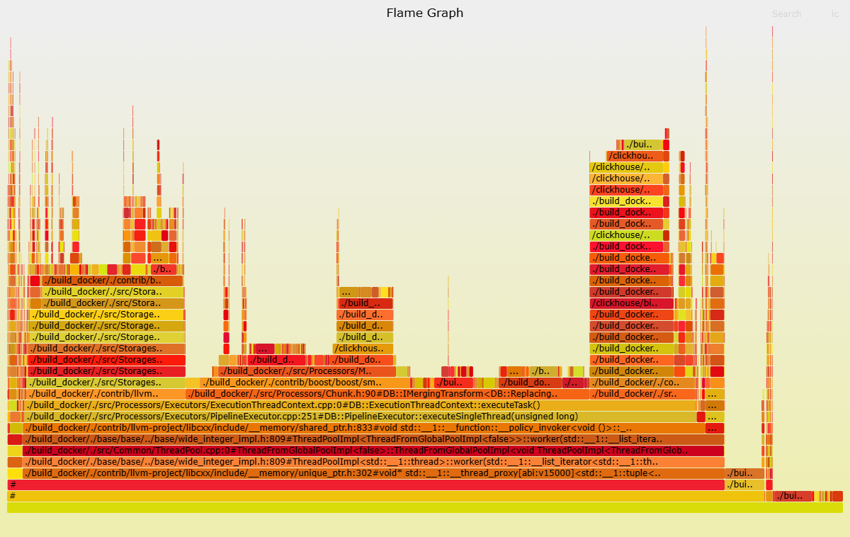
Analyze query_log
Run these queries simultaneously on both clusters to perform a top N comparison. Look for tables where CPU or memory usage is significantly higher on ApsaraDB for ClickHouse than on the self-managed cluster — those are your candidates.
High CPU or memory usage on a table doesn't always cause overall cluster degradation. It only suggests that table is more likely to be the source of the problem. Compare results between both clusters to confirm.
Locate tables with CPU issues
SELECT
    tables,
    first_value(query),
    count() AS cnt,
    groupArrayDistinct(normalizedQueryHash(query)) AS normalized_query_hash,
    sum(ProfileEvents.Values[indexOf(ProfileEvents.Names, 'UserTimeMicroseconds')]) AS sum_user_cpu,
    sum(ProfileEvents.Values[indexOf(ProfileEvents.Names, 'SystemTimeMicroseconds')]) AS sum_system_cpu,
    avg(ProfileEvents.Values[indexOf(ProfileEvents.Names, 'UserTimeMicroseconds')]) AS avg_user_cpu,
    avg(ProfileEvents.Values[indexOf(ProfileEvents.Names, 'SystemTimeMicroseconds')]) AS avg_system_cpu,
    sum(memory_usage) AS sum_memory_usage,
    avg(memory_usage) AS avg_memory_usage
FROM clusterAllReplicas(default, system.query_log)
WHERE (event_time > '2025-01-08 19:30:00') AND (event_time < '2025-01-08 20:30:00') AND (query_kind = 'Select')
GROUP BY tables
ORDER BY sum_user_cpu DESC
LIMIT 5
Locate tables with memory issues
SELECT
    tables,
    first_value(query),
    count() AS cnt,
    groupArrayDistinct(normalizedQueryHash(query)) AS normalized_query_hash,
    sum(ProfileEvents.Values[indexOf(ProfileEvents.Names, 'UserTimeMicroseconds')]) AS sum_user_cpu,
    sum(ProfileEvents.Values[indexOf(ProfileEvents.Names, 'SystemTimeMicroseconds')]) AS sum_system_cpu,
    avg(ProfileEvents.Values[indexOf(ProfileEvents.Names, 'UserTimeMicroseconds')]) AS avg_user_cpu,
    avg(ProfileEvents.Values[indexOf(ProfileEvents.Names, 'SystemTimeMicroseconds')]) AS avg_system_cpu,
    sum(memory_usage) AS sum_memory_usage,
    avg(memory_usage) AS avg_memory_usage
FROM clusterAllReplicas(default, system.query_log)
WHERE (event_time > '2025-01-08 19:30:00') AND (event_time < '2025-01-08 20:30:00') AND (query_kind = 'Select')
GROUP BY tables
ORDER BY sum_memory_usage
LIMIT 5
Replace event_time values with the time window when the performance issue occurred.
Step 2: Identify queries causing the performance bottleneck
After identifying the problematic table in Step 1, run the following queries to isolate the specific SQL statements causing the issue. Replace <AIM_TABLE> with the table name from Step 1, and update event_time to match your target time window.
Locate SQL queries that cause CPU issues
SELECT
    tables,
    first_value(query),
    count() AS cnt,
    normalizedQueryHash(query) AS normalized_query_hash,
    sum(ProfileEvents.Values[indexOf(ProfileEvents.Names, 'UserTimeMicroseconds')]) AS sum_user_cpu,
    sum(ProfileEvents.Values[indexOf(ProfileEvents.Names, 'SystemTimeMicroseconds')]) AS sum_system_cpu,
    avg(ProfileEvents.Values[indexOf(ProfileEvents.Names, 'UserTimeMicroseconds')]) AS avg_user_cpu,
    avg(ProfileEvents.Values[indexOf(ProfileEvents.Names, 'SystemTimeMicroseconds')]) AS avg_system_cpu,
    sum(memory_usage) AS sum_memory_usage,
    avg(memory_usage) AS avg_memory_usage
FROM clusterAllReplicas(default, system.query_log)
WHERE (event_time > '2025-01-08 19:30:00') AND (event_time < '2025-01-08 20:30:00') AND (query_kind = 'Select') AND has(tables, '<AIM_TABLE>')
GROUP BY
    tables,
    normalized_query_hash
ORDER BY sum_user_cpu DESC
LIMIT 5
Locate SQL queries that cause memory issues
SELECT
    tables,
    first_value(query),
    count() AS cnt,
    normalizedQueryHash(query) AS normalized_query_hash,
    sum(ProfileEvents.Values[indexOf(ProfileEvents.Names, 'UserTimeMicroseconds')]) AS sum_user_cpu,
    sum(ProfileEvents.Values[indexOf(ProfileEvents.Names, 'SystemTimeMicroseconds')]) AS sum_system_cpu,
    avg(ProfileEvents.Values[indexOf(ProfileEvents.Names, 'UserTimeMicroseconds')]) AS avg_user_cpu,
    avg(ProfileEvents.Values[indexOf(ProfileEvents.Names, 'SystemTimeMicroseconds')]) AS avg_system_cpu,
    sum(memory_usage) AS sum_memory_usage,
    avg(memory_usage) AS avg_memory_usage
FROM clusterAllReplicas(default, system.query_log)
WHERE (event_time > '2025-01-08 19:30:00') AND (event_time < '2025-01-08 20:30:00') AND (query_kind = 'Select') AND has(tables, 'AIM_TABLE')
GROUP BY
    tables,
    normalized_query_hash
ORDER BY sum_memory_usage
LIMIT 5
Step 3: Analyze SQL performance
Use EXPLAIN PIPELINE and system.query_log to understand why a specific query is slow.
Analyze the execution plan:
EXPLAIN PIPELINE <SQL with performance issues>For details on reading EXPLAIN output, see the ClickHouse EXPLAIN documentation.
Analyze execution metrics from query_log:
SELECT
    hostname() AS host,
    *
FROM clusterAllReplicas(`default`, system.query_log)
WHERE
    event_time > '2025-01-18 00:00:00'
    AND event_time < '2025-01-18 03:00:00'
    AND initial_query_id = '<INITIAL_QUERY_ID>'
    AND type = 'QueryFinish'
ORDER BY query_start_time_microseconds
Replace <INITIAL_QUERY_ID> with the query ID of the statement you want to investigate, and update event_time to cover the relevant time window.
Focus on these fields in the output:
| Field | What to look for |
|---|---|
ProfileEvents |
Detailed counters for CPU time, disk I/O, memory allocation, and network. Compares resource usage across nodes. See system events reference. |
Settings |
Configuration parameters active during the query. Helps identify settings that may be causing unexpected behavior. See settings reference. |
query_duration_ms |
Total query runtime. If a subquery is unusually slow, use its query_id to find its execution details in the log. To adjust log verbosity, see Configure config.xml parameters. |
If the metrics alone don't explain the performance degradation, pull the same query's execution information from the self-managed cluster and compare it side by side with the ApsaraDB for ClickHouse results. Differences in ProfileEvents values often reveal the root cause.
Step 4: Optimize SQL
After identifying the slow query, apply the relevant optimizations below. Most performance regressions after migration have a specific root cause — focus on the technique that matches your findings rather than applying all of them at once.
| Optimization | Description |
|---|---|
| Index optimization | Identify columns used frequently in WHERE clauses and create an index for them. |
| Data types | Use the most appropriate data types to reduce storage overhead and speed up reads. |
**Avoid SELECT *** |
Select only the columns you need to reduce I/O and network transfer. |
| Use primary key and index columns in WHERE | Filter on indexed columns to enable pruning. |
| Use PREWHERE | Move selective filter conditions to PREWHERE to reduce the data volume processed by subsequent stages. |
| Use GLOBAL JOIN for distributed tables | Replace regular JOIN with GLOBAL JOIN to avoid per-shard broadcast inefficiency. |
| Tune `max_threads` | Increasing max_threads uses more CPU cores, but setting it too high causes resource contention. See settings reference. |
| Create materialized views | For frequently executed complex queries with stable results, pre-aggregate with a materialized view. |
| Tune data compression | ClickHouse compresses data by default. Adjusting the compression algorithm and level can improve storage efficiency and query speed. |
| Expand the query cache | For stable, frequently repeated queries, increase uncompressed_cache_size to reduce recomputation. For parameter modification instructions, see Configure config.xml parameters. |