Partition pruning skips irrelevant partitions at query time, so AnalyticDB for PostgreSQL scans only the data that matches your filter conditions. This reduces I/O and improves query performance on large partitioned tables. When pruning works as expected, a query that filters on 1 of 12 months scans approximately 1/12 of the partitions.
AnalyticDB for PostgreSQL supports column-based partitioning. A fact table can be split into multiple partitions, and the system scans only the partitions that meet the specified query conditions.
AnalyticDB for PostgreSQL supports two types of partition pruning:
Static partition pruning — eliminates partitions before the query runs, based on constant filter expressions in the query. Check results with
EXPLAIN.Dynamic partition pruning — eliminates partitions during query execution, based on runtime values such as subquery results or JOIN inputs. Check results with
EXPLAIN ANALYZE.
Limitations
Partition pruning applies only to partitioned tables.
Static partition pruning supports the
=,>,>=,<,<=, andINpredicates on range or list partition columns. Operators such asLIKEand<>are not supported.Dynamic partition pruning supports only equivalence conditions (
=andIN) on partition columns.AnalyticDB for PostgreSQL V7.0 supports hash partitions. Hash partitions can be pruned only with equivalence conditions.
Pruning effectiveness depends on data distribution. If partition constraints cannot narrow the scan, the query falls back to a full table scan.
Static partition pruning
When a query's WHERE clause contains constant expressions on partition columns, the planner eliminates irrelevant partitions before building the query plan.
To check how many partitions are selected, run EXPLAIN and look for the Partition Selector node. The Partitions selected: N (out of M) field shows the result.
Examples
Example 1: Equality predicate
The following example creates a two-level partitioned table and runs a query with equality conditions on the partition columns.
-- Create a partitioned table
CREATE TABLE sales
  (id int, year int, month int, day int, region text)
DISTRIBUTED BY (id)
PARTITION BY RANGE (month)
  SUBPARTITION BY LIST (region)
    SUBPARTITION TEMPLATE (
    SUBPARTITION usa VALUES ('usa'),
    SUBPARTITION europe VALUES ('europe'),
    SUBPARTITION asia VALUES ('asia'),
    DEFAULT SUBPARTITION other_regions)
(START (1) END (13) EVERY (1),
DEFAULT PARTITION other_months );

-- Check the query plan
EXPLAIN
  SELECT * FROM sales
  WHERE year = 2008
    AND  month = 1
    AND  day = 3
    AND  region = 'usa';
The WHERE clause pins the query to level-1 partition month = 1 and level-2 subpartition region = 'usa'. Only 1 of 52 subpartitions is scanned.
Gather Motion 3:1  (slice1; segments: 3)  (cost=0.00..431.00 rows=1 width=24)
   ->  Sequence  (cost=0.00..431.00 rows=1 width=24)
         ->  Partition Selector for sales (dynamic scan id: 1)  (cost=10.00..100.00 rows=34 width=4)
               Partitions selected: 1 (out of 52)
         ->  Dynamic Seq Scan on sales (dynamic scan id: 1)  (cost=0.00..431.00 rows=1 width=24)
               Filter: ((year = 2008) AND (month = 1) AND (day = 3) AND (region = 'usa'::text))
Example 2: `IN` and `>=` predicates
EXPLAIN
  SELECT * FROM sales
  WHERE
  	month in (1,5)
    AND  region >= 'usa';
The IN predicate on month selects two level-1 partitions, and the >= predicate on region matches usa subpartitions in each. Six of 52 subpartitions are scanned.
                   								QUERY PLAN
----------------------------------------------------------------------------------------------
 Gather Motion 3:1  (slice1; segments: 3)  (cost=0.00..431.00 rows=1 width=24)
   ->  Sequence  (cost=0.00..431.00 rows=1 width=24)
         ->  Partition Selector for sales (dynamic scan id: 1)  (cost=10.00..100.00 rows=34 width=4)
               Partitions selected: 6 (out of 52)
         ->  Dynamic Seq Scan on sales (dynamic scan id: 1)  (cost=0.00..431.00 rows=1 width=24)
               Filter: ((month = ANY ('{1,5}'::integer[])) AND (region >= 'usa'::text))
Example 3: Unsupported predicate (`LIKE`)
LIKE is not supported for static partition pruning. All 52 partitions are scanned.
EXPLAIN
  SELECT * FROM sales
  WHERE region LIKE 'usa';
QUERY PLAN
----------------------------------------------------------------------------------------------
Gather Motion 3:1 (slice1; segments: 3) (cost=0.00..431.00 rows=1 width=24)
-> Sequence (cost=0.00..431.00 rows=1 width=24)
-> Partition Selector for sales (dynamic scan id: 1) (cost=10.00..100.00 rows=34 width=4)
Partitions selected: 52 (out of 52)
-> Dynamic Seq Scan on sales (dynamic scan id: 1) (cost=0.00..431.00 rows=1 width=24)
Filter: (region ~~ 'usa'::text)Dynamic partition pruning
For PREPARE-EXECUTE scenarios in which the partition constraint expression contains subqueries, the partition constraint cannot be resolved at plan time. The system uses external parameters and subquery responses to perform partition pruning during query execution, skipping irrelevant partitions at runtime.
To check how many partitions were actually scanned, run EXPLAIN ANALYZE and look for Partitions scanned: Avg N.0 (out of M) in the Dynamic Seq Scan node.
The plan-time estimate inPartition Selectormay showPartitions selected: 52 (out of 52)— this is expected. The planner cannot resolve runtime values before execution. ThePartitions scannedfield inEXPLAIN ANALYZEshows the actual runtime result.
Optimize JOIN operations with dynamic partition pruning
In data warehouse workloads, queries often join a large fact table with a small dimension table. If the join key matches the partition key of the fact table, dynamic partition pruning can significantly reduce the scan.
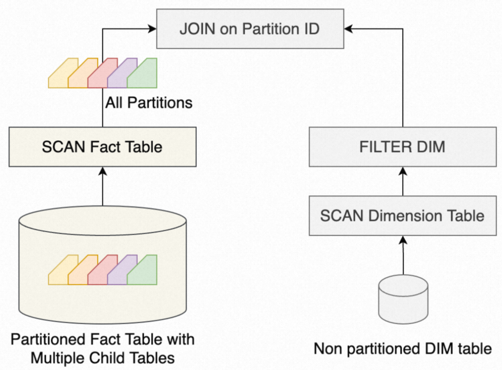
Without dynamic partition pruning, the system scans all partitions of the fact table before applying the JOIN filter:
With dynamic partition pruning enabled, the system first scans the dimension table, derives a partition filter from its values, and pushes that filter to the fact table's scan operator. Only matching partitions are read:
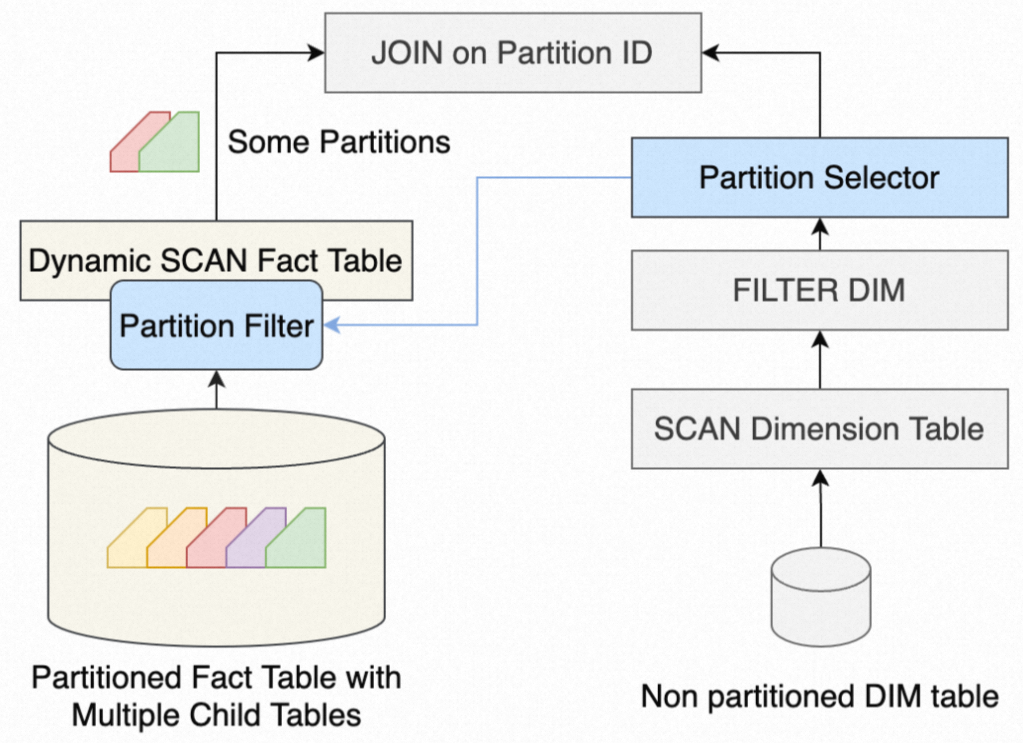
For joins between large partitioned fact tables and small dimension tables, use the partition key as the join key to enable dynamic partition pruning.
Examples
Example 1: Subquery in the WHERE clause
CREATE TABLE t1 (a int, b int);
INSERT INTO t1 VALUES (3,3), (5,5);

EXPLAIN ANALYZE
	SELECT * FROM sales
   WHERE month = (
     SELECT MIN(a) FROM t1 );
The subquery SELECT MIN(a) FROM t1 returns 3 at runtime. The system applies month = 3 as the partition constraint dynamically, scanning only the 4 partitions where month = 3.
Gather Motion 3:1  (slice3; segments: 3)  (cost=0.00..862.00 rows=1 width=24) (actual time=5.134..5.134 rows=0 loops=1)
 ->  Hash Join  (cost=0.00..862.00 rows=1 width=24) (never executed)
       Hash Cond: (sales.month = (min((min(t1.a)))))
       ->  Sequence  (cost=0.00..431.00 rows=1 width=24) (never executed)
             ->  Partition Selector for sales (dynamic scan id: 1)  (cost=10.00..100.00 rows=34 width=4) (never executed)
                   Partitions selected: 52 (out of 52)
             ->  Dynamic Seq Scan on sales (dynamic scan id: 1)  (cost=0.00..431.00 rows=1 width=24) (never executed)
                   Partitions scanned:  Avg 4.0 (out of 52) x 3 workers.  Max 4 parts (seg0).
       ->  Hash  (cost=100.00..100.00 rows=34 width=4) (actual time=0.821..0.821 rows=1 loops=1)
             ->  Partition Selector for sales (dynamic scan id: 1)  (cost=10.00..100.00 rows=34 width=4) (actual time=0.817..0.817 rows=1 loops=1)
                   ->  Broadcast Motion 1:3  (slice2)  (cost=0.00..431.00 rows=3 width=4) (actual time=0.612..0.612 rows=1 loops=1)
                         ->  Aggregate  (cost=0.00..431.00 rows=1 width=4) (actual time=1.204..1.205 rows=1 loops=1)
                               ->  Gather Motion 3:1  (slice1; segments: 3)  (cost=0.00..431.00 rows=1 width=4) (actual time=1.047..1.196 rows=3 loops=1)
                                     ->  Aggregate  (cost=0.00..431.00 rows=1 width=4) (actual time=0.012..0.012 rows=1 loops=1)
                                           ->  Seq Scan on t1  (cost=0.00..431.00 rows=1 width=4) (actual time=0.005..0.005 rows=2 loops=1)
The Partitions selected: 52 in the plan-time output is expected — the planner cannot resolve the subquery until runtime. The Avg 4.0 in Partitions scanned confirms pruning took effect.
Example 2: JOIN with a dimension table
EXPLAIN SELECT * FROM
	sales JOIN t1
   ON sales.month = t1.a
   WHERE sales.region = 'usa';
t1 contains two rows: (3,3) and (5,5). The join key month matches the partition key of sales. Dynamic partition pruning generates a filter month IN (3, 5) from t1's values, then applies the region = 'usa' filter within those partitions. Only 2 of 52 subpartitions are scanned.
QUERY PLAN
---------------------------------------------------------------------------------------------------------------
 Gather Motion 3:1  (slice2; segments: 3) (actual time=3.204..16.022 rows=6144 loops=1)
   ->  Hash Join (actual time=2.212..11.938 rows=6144 loops=1)
         Hash Cond: (sales.month = t1.a)
         Extra Text: (seg1)   Hash chain length 1.0 avg, 1 max, using 2 of 524288 buckets.
         ->  Sequence (actual time=0.317..4.197 rows=6144 loops=1)
               ->  Partition Selector for sales (dynamic scan id: 1) (never executed)
                     Partitions selected: 13 (out of 52)
               ->  Dynamic Seq Scan on sales (dynamic scan id: 1) (actual time=0.311..3.391 rows=6144 loops=1)
                     Filter: (region = 'usa'::text)
                     Partitions scanned:  Avg 2.0 (out of 52) x 3 workers.  Max 2 parts (seg0).
         ->  Hash (actual time=0.316..0.316 rows=2 loops=1)
               ->  Partition Selector for sales (dynamic scan id: 1) (actual time=0.208..0.310 rows=2 loops=1)
                     ->  Broadcast Motion 3:3  (slice1; segments: 3) (actual time=0.008..0.012 rows=2 loops=1)
                           ->  Seq Scan on t1 (actual time=0.004..0.004 rows=1 loops=1)
FAQ
How do I check whether partition pruning is working?
Run EXPLAIN and look for Partition Selector in the output. If it's present, partition pruning is active. For static pruning, check Partitions selected: N (out of M). For dynamic pruning, run EXPLAIN ANALYZE and check Partitions scanned: Avg N.0 (out of M) in the Dynamic Seq Scan node.
Do both the planner and ORCA support partition pruning?
Yes. Both the native PostgreSQL planner and ORCA support static and dynamic partition pruning. Their query plan output formats differ slightly, but both apply the same pruning logic.
Why isn't partition pruning working on my query?
Partition pruning requires that the query filter or join condition references the partition key. For static pruning, only =, >, >=, <, <=, and IN are supported — operators such as LIKE and <> will not trigger pruning. For dynamic pruning, only equivalence conditions (= and IN) work.