When a query is slow, knowing the total duration is not enough — you need to know where the time is spent and which part of the plan is the bottleneck. AnalyticDB for MySQL provides the SQL diagnostics feature that visualizes execution plans as interactive two-layer hierarchy charts, showing how the query executes across the cluster (the stage layer) and inside each stage (the operator layer). Each node surfaces duration, memory, row counts, and diagnostic recommendations, so you can pinpoint the slowest stage or operator without guessing.
How it works
The execution plan is a two-layer hierarchy chart:
Stage layer: Shows how the query is split into stages and how data moves between compute nodes.
Operator layer: Drills into a single stage to show each operator, its properties, and its resource usage.
Data flows from the bottom up in both layers. At the stage layer, scan stages read raw data first; intermediate stages process it; the root node at the top returns results to the client. The operator layer follows the same pattern: TableScan and RemoteSource operators at the bottom feed data upward to the root StageOutput or Output operator.
If the system detects a potential optimization for a stage or operator, a red icon with an exclamation point (!) appears on that node in the chart.
Stage layer
The stage layer gives you a cluster-wide view of query execution.
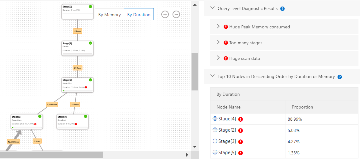
What each stage shows
Each rectangle represents a stage and displays:
Stage ID
Data output type (how data leaves this stage)
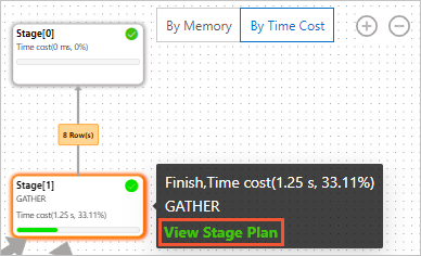
Duration or consumed memory — switch between them using By Duration and By Memory in the upper-right corner
Data flow between stages
The number on the line connecting two adjacent stages is the row count passing from the upstream stage to the downstream stage. A thicker line means more rows.
Data moves between stages using one of three methods:
| Data output method | Description |
|---|---|
| Broadcast | Each compute node in the upstream stage sends a full copy of its data to all compute nodes in the downstream stage. |
| Repartition | Each compute node in the upstream stage partitions its data according to specific rules and sends each partition to the designated compute nodes in the downstream stage. |
| Gather | Each compute node in the upstream stage sends all its data to a single compute node in the downstream stage. |
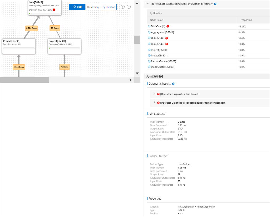
Top 10 nodes by duration or memory
The Top 10 Nodes in Descending Order by Duration or Memory panel on the right lists the stages with the largest share of total query duration or memory usage. By default, the panel sorts by duration. Select By Memory to switch to memory usage.
Stages that account for less than 1% of total duration or memory are excluded — these nodes are too small to affect overall query performance. The percentages shown may not sum to 100% due to differences in how metrics are collected.
Diagnostic results
Click a stage (for example, Stage[1]) to open its Diagnostic Results panel on the right. The panel contains:
Stage Diagnostics: A detailed description of detected issues for the stage — such as large amounts of broadcast data or data skew — along with optimization recommendations.
Operator Diagnostics: A summary of operators in the stage that have detected issues. For full details and optimization guidance, drill into the operator layer.
For a full list of stage diagnostic types, see Stage-level diagnostic results.
Stage statistics
The Statistics section below Diagnostic Results shows resource metrics for the selected stage.
| Metric | Description |
|---|---|
| Peak Memory | Maximum memory consumed by the stage. The unit auto-scales to Bytes, KB, MB, GB, or TB. |
| Cumulative Duration | Total execution time across all nodes, threads, and operators in the stage. The unit auto-scales to ms, s, m, or h. This value is a sum across parallel workers and cannot be compared directly to the total query duration. |
| Output Rows | Number of rows the stage produces. |
| Amount of Output Data | Volume of data the stage produces. The unit auto-scales to Bytes, KB, MB, GB, or TB. |
| Input Rows | Number of rows the stage receives. |
| Amount of Input Data | Volume of data the stage receives. The unit auto-scales to Bytes, KB, MB, GB, or TB. |
| Scanned Rows | Number of rows read from storage. Displayed only for stages that contain scan operators. |
| Scan Size | Volume of data read from storage. The unit auto-scales to Bytes, KB, MB, GB, or TB. Displayed only for stages that contain scan operators. |
Operator layer
The operator layer shows the execution plan inside a single stage, down to individual operators.
To open the operator layer, hover over any stage and click View Stage Plans in the tooltip that appears.
What each operator shows
Each rectangle represents an operator and displays:
Operator name and ID
Properties — for example, join conditions and algorithms of the JOIN operator
Duration or consumed memory — switch between them using By Duration and By Memory
Data flow between operators
The number on the line connecting two adjacent operators is the row count passing from the upstream operator to the downstream operator. A thicker line means more rows.
Top 10 nodes by duration or memory
The Top 10 Nodes in Descending Order by Duration or Memory panel lists the operators with the largest share of stage duration or memory usage. By default, the panel sorts by duration. Select By Memory to switch to memory usage. Operators that account for less than 1% of total duration or memory are excluded. The percentages may not sum to 100% due to differences in how metrics are collected.
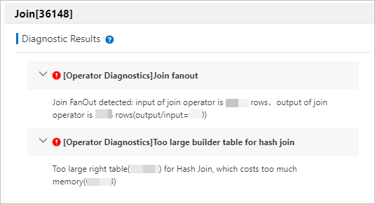
Diagnostic results
Click an operator (for example, Join[36184]) to open its Diagnostic Results panel. The panel shows the detected issues and optimization recommendations for that operator — such as data skew or an oversized right-hand table in a join.
For a full list of operator diagnostic types, see Operator-level diagnostic results.
Operator statistics
The Statistics section below Diagnostic Results shows resource metrics for the selected operator.
| Metric | Description |
|---|---|
| Peak Memory | Maximum memory consumed by the operator. The unit auto-scales to Bytes, KB, MB, GB, or TB. |
| Time Consumed | Average execution time of the operator at its actual concurrency level. The unit auto-scales to ms, s, m, or h. This value can be compared directly to the total query duration. |
| Output Rows | Number of rows the operator produces. |
| Amount of Output Data | Volume of data the operator produces. The unit auto-scales to Bytes, KB, MB, GB, or TB. |
| Input Rows | Number of rows the operator receives. |
| Amount of Input Data | Volume of data the operator receives. The unit auto-scales to Bytes, KB, MB, GB, or TB. |
| Builder Statistics | Build-phase statistics for JOIN operators, including builder type, peak memory, duration, input rows, output rows, and data volume. Three builder types are available: HashBuilder (builds hash tables for hash joins), SetBuilder (builds sets for semi joins), and NestLoopBuilder (handles nested loop joins). Displayed only for JOIN operators. |
| Properties | Operator-specific configuration details. For JOIN operators, this includes the join type and join method. For the full list of operator properties, see Operators. |
Common performance patterns
The following patterns commonly appear in execution plans for slow queries. Use the stage and operator layers to identify them.
Large broadcast data
Broadcast transfers a full copy of upstream data to every downstream compute node. If the upstream stage is large, this significantly increases network traffic and memory usage. Look for stages with Broadcast output and high row counts on the connecting line. The Stage Diagnostics panel flags this issue and provides optimization recommendations.
Data skew
Data skew occurs when one compute node processes far more rows than others. In the stage layer, a skewed stage typically shows high Cumulative Duration relative to other stages of similar function. The Diagnostic Results panel identifies skew and suggests optimization solutions.
Oversized join right-hand table
For JOIN operators, the right-hand table is loaded into memory during the build phase. An oversized right-hand table causes high Peak Memory on the JOIN operator. Check Builder Statistics in the operator's Statistics section to see build-phase memory and row counts. The Diagnostic Results panel flags this when detected.