By Digoal
With the technological advancements, futuristic scenes depicted in science fiction movies are gradually becoming a reality. Vendors in military and civilian industries, including many automobile vendors and high-tech companies, are committed to developing driverless cars and unmanned aerial vehicles (UAVs).
Pilotless driving has a wide range of applications in various industries, for example, the express delivery industry. When time is ripe, couriers may no longer be needed so that they can be free from trivial parcel delivery work and have more time to enjoy a life empowered by science and technology.
Navigation is essential for driverless cars and UAVs, while location information is essential for navigation. Location information consists of a countless number of points. The precision increases as the number of points increases. Consider photos shot by mobile phones as an analogy. Early mobile phone cameras had low pixel quality and rough image sensors. As a result, photos shot with those mobile phones are not nearly as clear as photos shot with modern mobile phones.

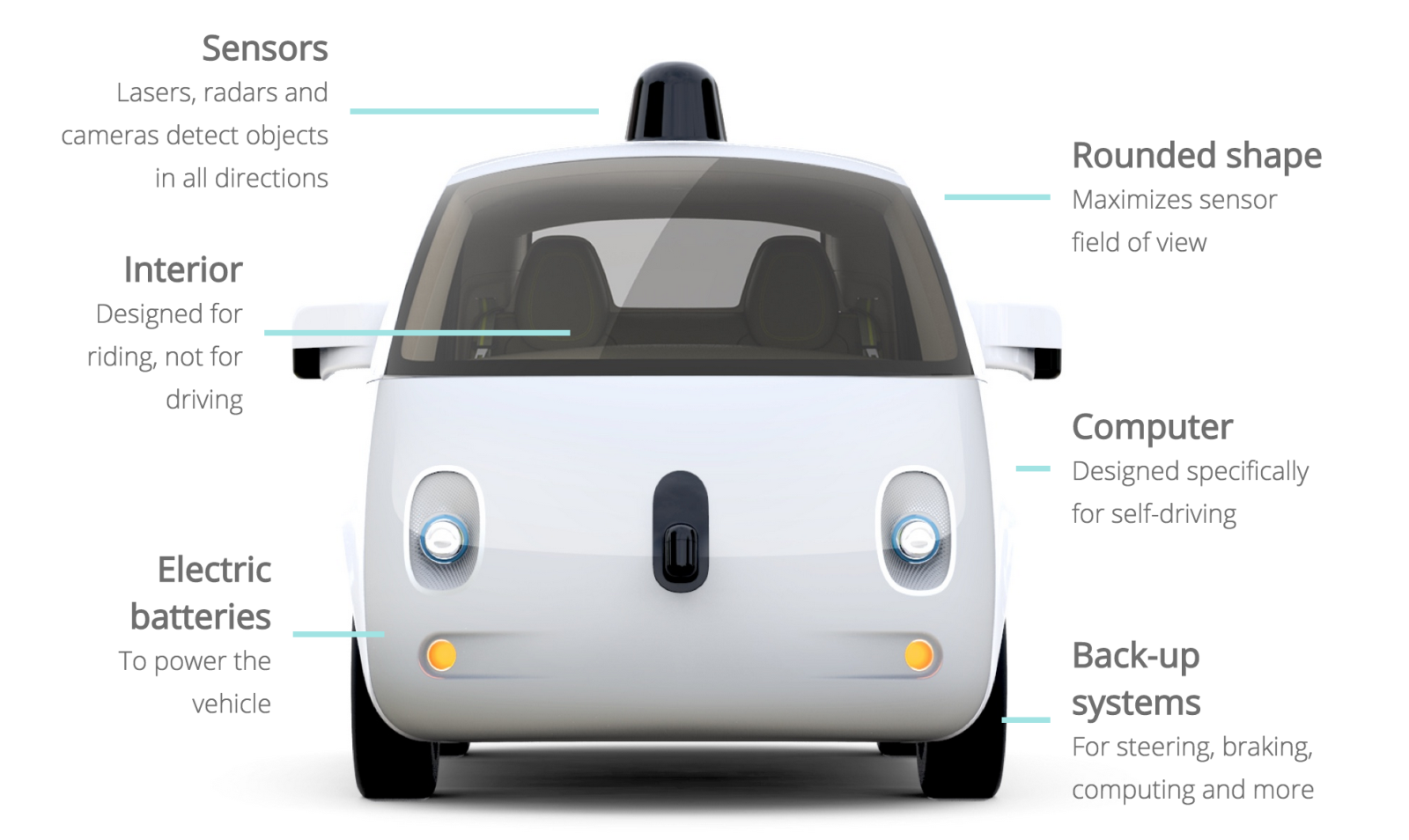
Besides, the point density needs to meet a specified threshold for pilotless driving to be usable. Assume that each square meter represents one point. An area of 1 square kilometer needs 1 million points. The scale of 1 meter certainly is coarse-grained. There is no need to cover all points as driving alone, and only the road area needs to be covered.
For example, how many points are required to describe a six-lane two-way road that is 100 kilometers long and 25 meters wide? If each square meter needs one point, 2.5 million points are needed. If an area of 1 square meter is divided into 10 grids and each grid needs one point, 25 million points are needed. If an area of 1 square meter is divided into 100 grids and each grid needs one point, 250 million points are needed. PostgreSQL PostGIS can achieve finer data granules. It uses longitude and latitude (float8, float8) to represent a point instead of a grid. In some databases, points are represented by using geohash values, but this compromises precision.
After knowing the approximate point volume, how can we implement pilotless driving by using the points?
For simplicity, a point array is referred to as a point cloud. After the starting point and pilotless driving, the path is determined for a vehicle, points for all related roads need to be loaded into the vehicle. Each point needs to include other attributes besides the location, for example, information indicating a maintenance hole cover, a pit, whether the road is a cement road or a tarmac road, traffic lights, road shoulder, etc. Other specific fields can store these attributes.
The point cloud is used as a location and attribute data in conjunction with the autopiloting software.
PostGIS is a popular GIS data management extension widely applied in astronomy, scientific research, military, and the internet. Alibaba Cloud's ApsaraDB RDS for PostgreSQL has integrated PostGIS. You can choose ApsaraDB RDS for PostgreSQL or install PostgreSQL and PostGIS.
Store data in PostgreSQL and use the geometry data type and GiST indexes to achieve optimal retrieval performance.
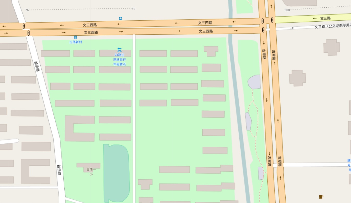
Several points represent every road. When the vehicle starts, positioning is performed, nearby points are loaded, and points intersecting with the road polygon are returned. The point cloud's resolution (density) needs to meet a very high standard to enable pilotless driving. As described above, for a six-lane two-way road that is 100 kilometers long and 25 meters wide, when an area of 1 square meter is represented by using 100 points, the road needs 250 million points.
If a pilotless vehicle travels at a speed of 1 kilometer/minute (that is, 60 kilometers/hour), the loading speed needs to reach at least 2.5 million points/minute.
First, use one record to represent one point (optimization is described below).
1) Create a table schema (using ApsaraDB RDS for PostgreSQL as an example).
create extension postgis;  -- 创建postgis插件

postgres=# create table cloudpoint_test(
  id serial primary key,  -- 主键
  loc geometry,        -- 经纬度(或point)
  other text           -- 其他属性
);
CREATE TABLE
2) Create a GiST index.
postgres=# create index idx on cloudpoint_test using gist(loc) with (buffering=on);
CREATE INDEX 1) Insert test data of 100 million points with a 50-thread concurrency. The area covers 100 million random points with 10,000 points in length and 10,000 points in width.
vi ins.sql

insert into cloudpoint_test (loc,other) values (st_makepoint(random()*10000, random()*10000) , 'test');
2) Check the data insertion performance. About 166,000 records are inserted per second.
pgbench -M prepared -n -r -P 1 -f ./ins.sql -c 50 -j 50 -t 2000000

transaction type: Custom query
scaling factor: 1
query mode: prepared
number of clients: 50
number of threads: 50
number of transactions per client: 2000000
number of transactions actually processed: 100000000/100000000
latency average: 0.298 ms
latency stddev: 0.854 ms
tps = 166737.438650 (including connections establishing)
tps = 166739.148413 (excluding connections establishing)
statement latencies in milliseconds:
0.297896 insert into cloudpoint_test (loc,other) values (st_makepoint(random()*10000, random()*10000) , 'test'); 1) Customize a point search function as follows.
create or replace function ff(geometry, float8, int) returns setof record as $$
declare
  v_rec record;
  v_limit int := $3;
begin
  set local enable_seqscan=off;   -- 强制索引, 扫描行数够就退出.
  for v_rec in
    select *,
    ST_Distance ( $1, loc ) as dist
    from cloudpoint_test
    order by loc <-> $1           -- 按距离顺序由近到远返回
  loop
    if v_limit <=0 then           -- 判断返回的记录数是否达到LIMIT的记录数
      raise notice '已经取足limit设置的 % 条数据, 但是距离 % 以内的点可能还有.', $3, $2;
      return;
    end if;
    if v_rec.dist > $2 then       -- 判断距离是否大于请求的距离
      raise notice '距离 % 以内的点已输出完毕', $2;
      return;
    else
      return next v_rec;
    end if;
    v_limit := v_limit -1;
  end loop;
end;
$$ language plpgsql strict volatile;
2) Use the following SQL query statement.
The statement searches for points within 100 points away from st_makepoint(1500,1500) and returns a maximum of 10,000 points by distance in ascending order.
postgres=# select * from ff(st_makepoint(1500,1500), 100, 10000) as t (id int, loc geometry, other text, dist float8);
NOTICE:  已经取足limit设置的 10000 条数据, 但是距离 100 以内的点可能还有.
    id     |                    loc                     | other |       dist
-----------+--------------------------------------------+-------+-------------------
  54528779 | 01010000000000EFF6307297400000010D306E9740 | test  | 0.710901366481036
  52422694 | 01010000000080EE51B171974000003DE6256D9740 | test  | 0.829108575682196
  20123322 | 0101000000000074AD5C6F97400000C766CE739740 | test  |   0.9648380442046
  58784192 | 010100000000803A65F4749740008012FDD8709740 | test  |  1.25666215808279
......1) Search for 200,000 points within 1,000 points away from st_makepoint(5000,5000) and return the points by distance in ascending order.
Response time: 1 second
explain (analyze,verbose,timing,costs,buffers) select * from ff(st_makepoint(5000,5000), 1000, 200000) as t(id int, loc geometry, other text, dist float8);

NOTICE:  已经取足limit设置的 200000 条数据, 但是距离 1000 以内的点可能还有.
                                                       QUERY PLAN
------------------------------------------------------------------------------------------------------------------------
 Function Scan on public.ff t  (cost=0.25..10.25 rows=1000 width=76) (actual time=917.748..945.838 rows=200000 loops=1)
   Output: id, loc, other, dist
   Function Call: ff('0101000000000000000088B340000000000088B340'::geometry, 1000::double precision, 200000)
   Buffers: shared hit=201288, temp read=1418 written=1417
 Planning time: 0.057 ms
 Execution time: 959.534 ms
(6 rows)
2) Search for 1 million points within 2,000 points away from st_makepoint(5000,5000) and return the points by distance in ascending order.
Response time: 10 seconds
explain (analyze,verbose,timing,costs,buffers) select * from ff(st_makepoint(5000,5000), 2000, 1000000) as t(id int, loc geometry, other text, dist float8);

NOTICE:  已经取足limit设置的 1000000 条数据, 但是距离 2000 以内的点可能还有.
                                                        QUERY PLAN
---------------------------------------------------------------------------------------------------------------------------
 Function Scan on public.ff t  (cost=0.25..10.25 rows=1000 width=76) (actual time=8867.007..9006.401 rows=1000000 loops=1)
   Output: id, loc, other, dist
   Function Call: ff('0101000000000000000088B340000000000088B340'::geometry, 2000::double precision, 1000000)
   Buffers: shared hit=1006220, temp read=7082 written=7081
 Planning time: 0.059 ms
 Execution time: 9074.267 ms
(6 rows)
3) Search for 5 million points within 3,000 points away from st_makepoint(5000,5000) and return the points by distance in ascending order.
Response time: 43 seconds
explain (analyze,verbose,timing,costs,buffers) select * from ff(st_makepoint(5000,5000), 3000, 5000000) as t(id int, loc geometry, other text, dist float8);

NOTICE:  已经取足limit设置的 5000000 条数据, 但是距离 3000 以内的点可能还有.
                                                         QUERY PLAN
-----------------------------------------------------------------------------------------------------------------------------
 Function Scan on public.ff t  (cost=0.25..10.25 rows=1000 width=76) (actual time=42168.038..42861.462 rows=5000000 loops=1)
   Output: id, loc, other, dist
   Function Call: ff('0101000000000000000088B340000000000088B340'::geometry, 3000::double precision, 5000000)
   Buffers: shared hit=5030448, temp read=35402 written=35401
 Planning time: 0.060 ms
 Execution time: 43201.879 ms
(6 rows)
The performance data looks good, right? However, we should not stop here. We can optimize performance. Keep reading.
Three aspects bottleneck the performance.
Because of the need to return a large number of records, PostgreSQL also has a large number of callbacks to return records, resulting in high overhead.
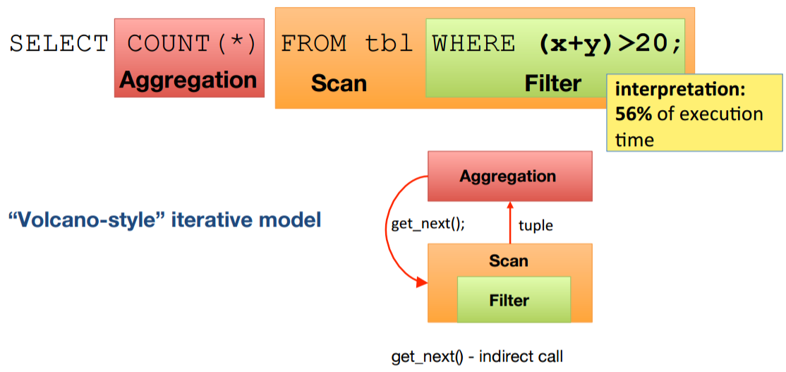
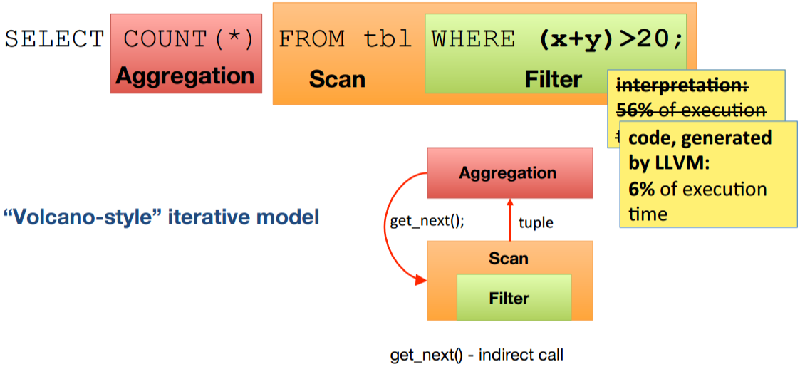
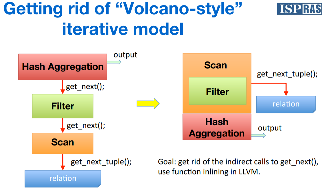
This can be viewed by using perf.
perf record -ag -p $PID

perf report -ag --stdio Point data may be collected randomly. Therefore, data at the heap storage layer is non-ordered, and no specific order is used to search for points near a certain point. The discrete I/O requests result in heap I/O amplification.
The discrete degree problem of index entries exists even when GiST indexes are created. For more information, see https://www.postgresql.org/docs/10.0/static/gist-implementation.html
From version 9.2, PostgreSQL supports a more efficient method to build GiST indexes based on buffering, which can dramatically reduce the number of random I/Os needed for non-ordered data sets.
For well-ordered data sets, the benefit is smaller or non-existent because only a small number of pages receive new tuples at a time, and those pages fit in cache even if the index as a whole does not.
How to optimize point cloud search to address these three issues?
If there are too many callbacks, returning or processing too many records may bottleneck the performance. Three optimization methods are available to address this scenario.
Previously, an area of 1 square meter is divided into 100 points (100 records). If every area of 1 square meter is regarded as one grid, and the 100 records are aggregated into one record, the total number of records is reduced by 100 times.
The 100 million records are reduced to 1 million records, and the number of user requests is also reduced by 100 times.
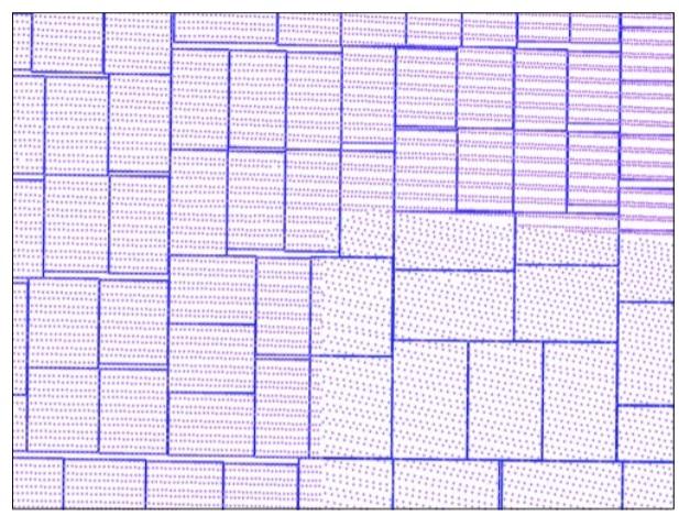
The table schema after aggregation is as follows.
postgres=# create table cloudpoint_test_agg(
  id serial primary key,        -- 主键
  loc_box geometry,          -- 格子(闭合多边形), 表示一个范围内的点
  loc_agg geometry[],        -- 经纬度数组(或point数组)
  other_agg text[]           -- 其他属性数组
);
CREATE TABLE

create index idx_cloudpoint_test_agg_1 on cloudpoint_test_agg using gist(loc_box) with (buffering=on);
How to Implement Aggregation?
First, convert the road into adjacent hexagon grids.
The converted road information is as follows.
create table cloudpoint_test_grid(
  id serial primary key,    -- 六边形ID
  loc_box geometry     -- 单个六边形
);
Join the grids and point cloud data into aggregated data.
insert into cloudpoint_test_agg (loc_box,loc_agg,other_agg)
  select t1.loc_box, array_agg(t2.loc) as loc_agg, array_agg(t2.other) as other_agg from
    cloudpoint_test_grid t1 join cloudpoint_test t2
    on (ST_Contains(t1.loc_box, t2.loc)) group by t1.loc_box;
Example:
In this example, a standard square area of ((0,0),(10000,10000)) is divided into grids by taking the following steps:
Divide the square into grids, each with an area of 100*100.

Reference: http://postgis.net/docs/manual-2.3/ST_MakeBox2D.html
do language plpgsql $$
declare
  x int;
  y int;
begin
  for x in select generate_series(0,10000,100) loop
    for y in select generate_series(0,10000,100) loop
      insert into cloudpoint_test_grid(loc_box) values (ST_MakeBox2D( st_makepoint(x,y), st_makepoint(x+100, y+100) ));
    end loop;
  end loop;
end;
$$;
postgres=# select * from cloudpoint_test_grid;
  id   |                                                                                          loc_box
-------+--------------------------------------------------------------------------------------------------------------------------------------------------------------------------------------------
     1 | 010300000001000000050000000000000000000000000000000000000000000000000000000000000000005940000000000000594000000000000059400000000000005940000000000000000000000000000000000000000000000000
     2 | 010300000001000000050000000000000000000000000000000000594000000000000000000000000000006940000000000000594000000000000069400000000000005940000000000000594000000000000000000000000000005940
     3 | 010300000001000000050000000000000000000000000000000000694000000000000000000000000000C0724000000000000059400000000000C072400000000000005940000000000000694000000000000000000000000000006940
     4 | 0103000000010000000500000000000000000000000000000000C07240000000000000000000000000000079400000000000005940000000000000794000000000000059400000000000C0724000000000000000000000000000C07240

......
Generate aggregated data.
insert into cloudpoint_test_agg (loc_box,loc_agg,other_agg)
  select t1.loc_box, array_agg(t2.loc) as loc_agg, array_agg(t2.other) as other_agg from
    cloudpoint_test_grid t1 join cloudpoint_test t2
    on (ST_Contains(t1.loc_box, t2.loc)) group by t1.loc_box;

INSERT 0 10000

select count(*) from cloudpoint_test_agg;
10000
Use the following function to search the aggregated point cloud data for nearby points.
create or replace function ff1(geometry, float8, int) returns setof record as $$
declare
  v_rec record;
  v_limit int := $3;
begin
  set local enable_seqscan=off;   -- 强制索引, 扫描行数够就退出.
  for v_rec in
    select *,
    ST_Distance ( $1, loc_box ) as dist
    from cloudpoint_test_agg
    order by loc_box <-> $1           -- 按距离顺序由近到远返回
  loop
    if v_limit <=0 then           -- 判断返回的记录数是否达到LIMIT的记录数
      raise notice '已经取足limit设置的 % 条数据, 但是距离 % 以内的点可能还有.', $3, $2;
      return;
    end if;
    if v_rec.dist > $2 then       -- 判断距离是否大于请求的距离
      raise notice '距离 % 以内的点已输出完毕', $2;
      return;
    else
      return next v_rec;
    end if;
    v_limit := v_limit - array_length(v_rec.loc_agg, 1);  -- 扣减grid内的point个数
  end loop;
end;
$$ language plpgsql strict volatile;
Alternative Aggregation Method
Use the st_geohash(geometry) function to extract geohash values of points and perform aggregation based on the geohash values' prefixes.
The geohash values of adjacent points are also adjacent.
Sample SQL Query Statement After Aggregation
The statement searches for points within 100 points away from st_makepoint(1500,1500) and returns a maximum of 10,000 points by distance in ascending order.
postgres=# select * from ff1(st_makepoint(1500,1500), 100, 10000) as t (id int, loc_box geometry, loc_agg geometry[], other_agg text[], dist float8);Speed Test After Aggregation
1) Search for 200,000 points within 1,000 points away from st_makepoint(5000,5000) and return the points by distance in ascending order.
Response time: 15 milliseconds
postgres=# explain (analyze,verbose,timing,costs,buffers) select * from ff1(st_makepoint(5000,5000), 1000, 200000) as t (id int, loc_box geometry, loc_agg geometry[], other_agg text[], dist float8);
NOTICE:  已经取足limit设置的 200000 条数据, 但是距离 1000 以内的点可能还有.
                                                     QUERY PLAN
--------------------------------------------------------------------------------------------------------------------
 Function Scan on public.ff1 t  (cost=0.25..10.25 rows=1000 width=108) (actual time=15.642..15.643 rows=20 loops=1)
   Output: id, loc_box, loc_agg, other_agg, dist
   Function Call: ff1('0101000000000000000088B340000000000088B340'::geometry, 1000::double precision, 200000)
   Buffers: shared hit=465
 Planning time: 0.082 ms
 Execution time: 15.670 ms
(6 rows)
2) Search for 1 million points within 2,000 points away from st_makepoint(5000,5000) and return the points by distance in ascending order.
Response time: 63 milliseconds
postgres=# explain (analyze,verbose,timing,costs,buffers) select * from ff1(st_makepoint(5000,5000), 2000, 1000000) as t (id int, loc_box geometry, loc_agg geometry[], other_agg text[], dist float8);
NOTICE:  已经取足limit设置的 1000000 条数据, 但是距离 2000 以内的点可能还有.
                                                     QUERY PLAN
---------------------------------------------------------------------------------------------------------------------
 Function Scan on public.ff1 t  (cost=0.25..10.25 rows=1000 width=108) (actual time=63.287..63.296 rows=100 loops=1)
   Output: id, loc_box, loc_agg, other_agg, dist
   Function Call: ff1('0101000000000000000088B340000000000088B340'::geometry, 2000::double precision, 1000000)
   Buffers: shared hit=2143
 Planning time: 0.057 ms
 Execution time: 63.322 ms
(6 rows)
3) Search for 5 million points within 3,000 points away from st_makepoint(5000,5000) and return the points by distance in ascending order.
Response time: 312 milliseconds
postgres=# explain (analyze,verbose,timing,costs,buffers) select * from ff1(st_makepoint(5000,5000), 3000, 5000000) as t (id int, loc_box geometry, loc_agg geometry[], other_agg text[], dist float8);
NOTICE:  已经取足limit设置的 5000000 条数据, 但是距离 3000 以内的点可能还有.
                                                      QUERY PLAN
-----------------------------------------------------------------------------------------------------------------------
 Function Scan on public.ff1 t  (cost=0.25..10.25 rows=1000 width=108) (actual time=312.315..312.394 rows=501 loops=1)
   Output: id, loc_box, loc_agg, other_agg, dist
   Function Call: ff1('0101000000000000000088B340000000000088B340'::geometry, 3000::double precision, 5000000)
   Buffers: shared hit=10729
 Planning time: 0.077 ms
 Execution time: 312.463 ms
(6 rows)
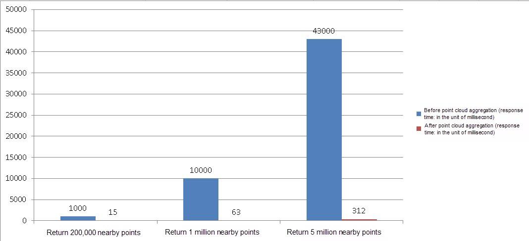
Comparison of performance before and after aggregation:
pgPointcloud is a PostgreSQL extension for storing point cloud (LiDAR) data. It provides features similar to PostGIS raster data and also more extended features.

LiDAR in PostgreSQL with PointCloud
A LiDAR sensor can rapidly generate millions of points while scanning a space. Each point may include other dimensional information besides the X, Y, and Z coordinate values, such as time, RGB values, and other attributes. Points may also be returned in batches.
As a result, LiDAR sensors' reported data is not stored in a fixed data type. pgPointcloud uses the "schema document" type to describe LiDAR sensors' reported data in a format like that in the PDAL repository.
Each point includes information about several dimensions. Each dimension's information may be on any data type. Therefore, the point data is of a composite type.
As described by the official documentation of PostgreSQL, LIDAR sensors quickly produce millions of points with large numbers of variables measured on each point. The challenge for a point cloud database extension is efficiently storing this data while allowing high fidelity access to the many variables stored.
Much of the complexity in handling LIDAR comes from the need to deal with multiple variables per point. The variables captured by LIDAR sensors vary by sensor and capture process. Some data sets might contain only X/Y/Z values. Others will contain dozens of variables: X, Y, Z; intensity and return number; red, green, and blue values; return times; and many more.
There is no consistency in how variables are stored: intensity might be stored in a 4-byte integer or a single byte; X/Y/Z might be double, or they might be scaled 4-byte integers. PostgreSQL Pointcloud deals with all this variability by using a "schema document" to describe any particular LIDAR point's contents.
Each point contains many dimensions, and each dimension can be of any data type, with scaling and/or offsets applied to move between the actual value and the value stored in the database.
The schema document format used by PostgreSQL Pointcloud is the same one used by the PDAL library.
pgPointcloud is an extension especially designed for processing LiDAR data. We recommend that you use pgpointcloud.
The overhead incurred by the get next tuple method may be increased due to a large number of processed records. To resolve this issue, reduce the callback overhead using code generation or a vector calculation method.
GiST index optimization helps reduce the number of fragments. To enable this feature, simply set the buffering parameter of GiST to "on". You can specify this parameter when creating a GiST index.
create index idx_cloudpoint_test_agg_1 on cloudpoint_test_agg using gist(loc_box) with (buffering=on);
create index idx_cloudpoint_test_1 on cloudpoint_test using gist(loc) with (buffering=on); When a large number of records need to be returned, the records can be returned in batches or a stream.
Records can be returned in a stream by using two methods: using cursors or asynchronous messages.
begin;

declare cur1 cursor for select * from (select *, ST_Distance ( st_makepoint(5000,5000), loc ) as dist from cloudpoint_test order by st_makepoint(5000,5000) <-> loc ) t where dist < 1000;

fetch 100 from cur1;

fetch ...;

-- 客户端接收到足够的数据,或者距离超出后,不再接收,关闭游标,退出事务。

close cur1;

end;
For more information, see the PostgreSQL driver of your programming language, for example, JDBC for PostgreSQL or libpq.
Session 1 monitors the channel.
listen abcd; Session 2 initiates a request to send an asynchronous message to the monitored channel.
create or replace function ff(geometry, float8, int, text) returns void as $$
declare
  v_rec record;
  v_limit int := $3;
begin
  set local enable_seqscan=off;   -- 强制索引, 扫描行数够就退出.
  for v_rec in
    select *,
    ST_Distance ( $1, loc ) as dist
    from cloudpoint_test
    order by loc <-> $1           -- 按距离顺序由近到远返回
  loop
    if v_limit <=0 then           -- 判断返回的记录数是否达到LIMIT的记录数
      raise notice '已经取足limit设置的 % 条数据, 但是距离 % 以内的点可能还有.', $3, $2;
      return;
    end if;
    if v_rec.dist > $2 then       -- 判断距离是否大于请求的距离
      raise notice '距离 % 以内的点已输出完毕', $2;
      return;
    else
      -- return next v_rec;
      perform pg_notify ($4, v_rec::text);
    end if;
    v_limit := v_limit -1;
  end loop;
end;
$$ language plpgsql strict volatile;
Session 2 initiates a search request.
postgres=# select ff(st_makepoint(5000,5000), 1000, 10, 'abcd');
NOTICE:  已经取足limit设置的 10 条数据, 但是距离 1000 以内的点可能还有.
 ff
----

(1 row)
Session 1 receives the message from the channel asynchronously.
Asynchronous notification "abcd" with payload "(38434407,01010000000060763E6E87B34000C0028CC587B340,test,0.613437682476958)" received from server process with PID 36946.
Asynchronous notification "abcd" with payload "(41792090,0101000000006008B91F88B3400000D5D13B87B340,test,0.776283650707887)" received from server process with PID 36946.
Asynchronous notification "abcd" with payload "(90599062,0101000000002057B2A888B34000C093516E88B340,test,0.787366330405518)" received from server process with PID 36946.
Asynchronous notification "abcd" with payload "(69482516,01010000000000A574AE88B34000601AEBA888B340,test,0.948568992176712)" received from server process with PID 36946.
Asynchronous notification "abcd" with payload "(12426846,0101000000006075D49188B34000E0E8E70487B340,test,1.13425697837729)" received from server process with PID 36946.
Asynchronous notification "abcd" with payload "(98299759,0101000000004054059388B340006014ED1089B340,test,1.21096126708341)" received from server process with PID 36946.
Asynchronous notification "abcd" with payload "(31175773,010100000000C03179EE88B34000A03E0C1B87B340,test,1.29136079279649)" received from server process with PID 36946.
Asynchronous notification "abcd" with payload "(11651191,01010000000080C6634C87B34000E0A4852689B340,test,1.34753214416354)" received from server process with PID 36946.
Asynchronous notification "abcd" with payload "(50248773,010100000000C064B3A686B34000809FA0F487B340,test,1.34955653568245)" received from server process with PID 36946.
Asynchronous notification "abcd" with payload "(28170573,010100000000608F958B86B34000C051C1F587B340,test,1.45529948415963)" received from server process with PID 36946.
For more information, see the PostgreSQL driver of your programming language, for example, JDBC for PostgreSQL or libpq.
Record the generated point cloud data into the heap table in order based on the geographical location information. In this way, you can narrow down the data blocks that need to be accessed in the heap table when searching data within a specified range.
When playing with Lego bricks, we arrange bricks with different shapes into different boxes. When a certain shaped brick is required, we can easily find it in its corresponding box without rummaging through other boxes.
Like playing with Lego bricks, store data based on the query requests to reduce the heap I/O overhead during index queries.
PostGIS is a spatial data management extension for PostgreSQL. It can manage various data types, such as geographical locations, multi-dimensional data, raster data, and topologies. It performs space calculation, superposition calculation, point and plane queries, and other spatial data-related computations.
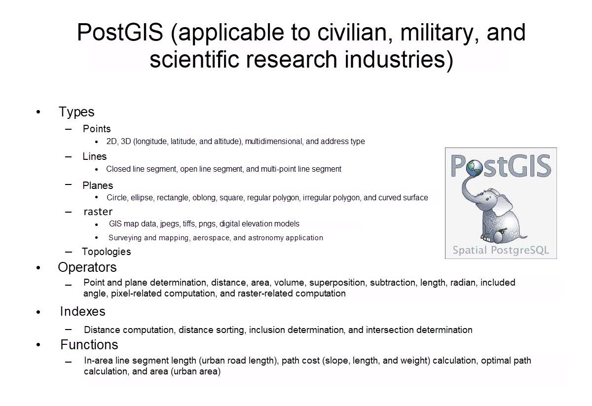
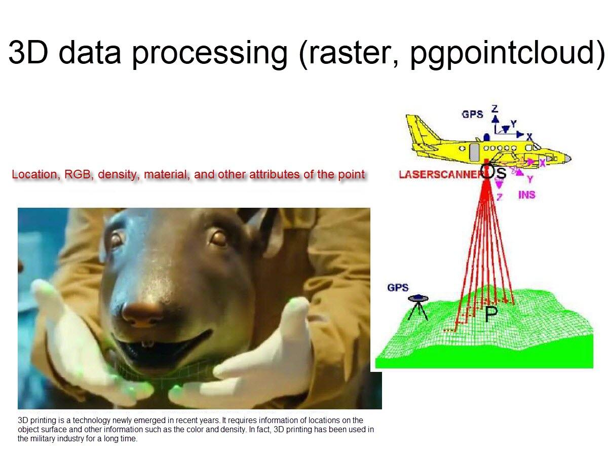
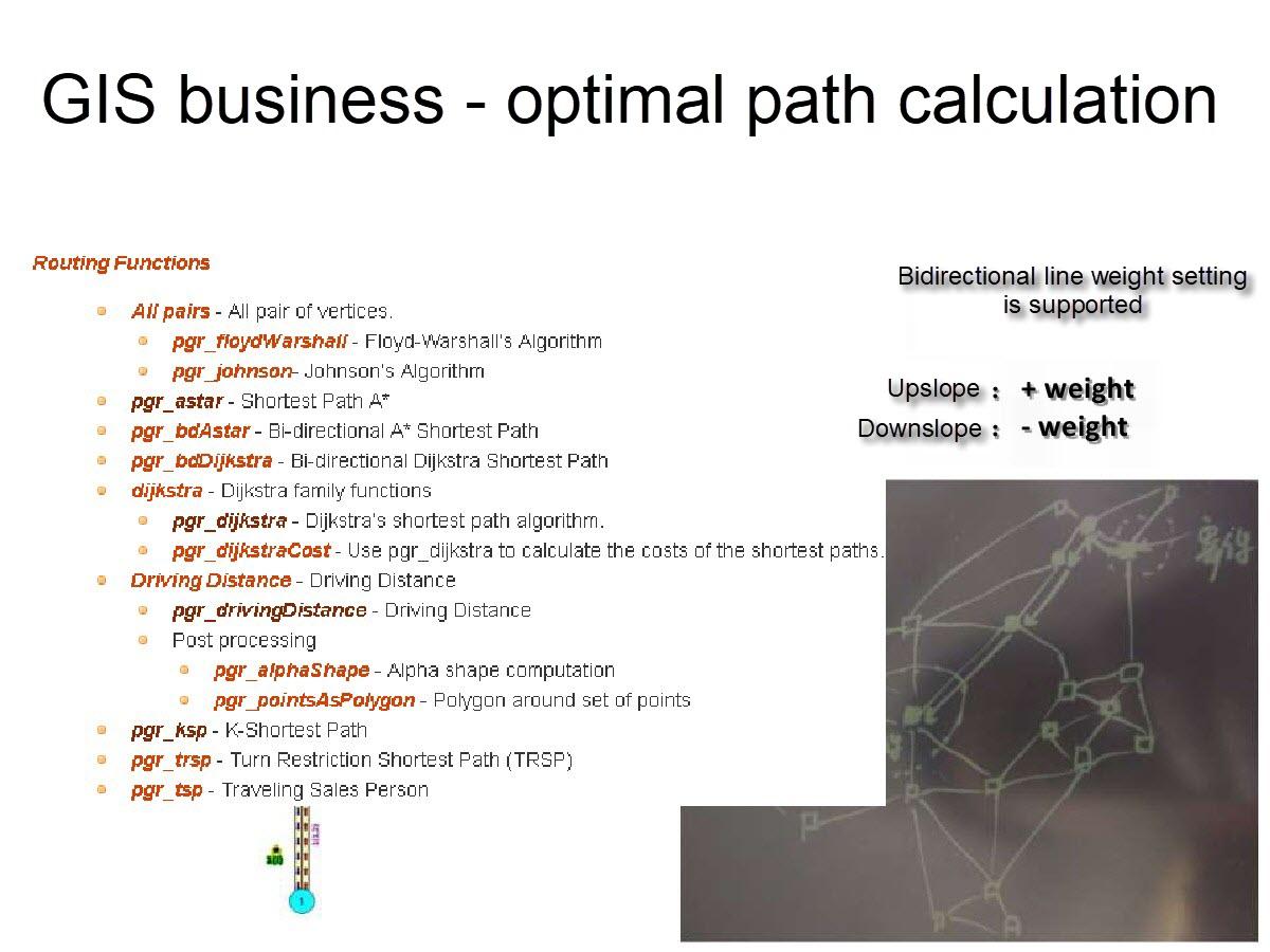

The rise of pilotless driving and logistics delivery robots has posed considerable challenges to conventional GIS databases:
1) First, in terms of data volume, when each area of 1 square meter is divided into 100 points, 250 million points are needed for a six-lane two-way road that is 100 kilometers long and 25 meters wide.
2) Second, in terms of data attributes, not only the longitude, latitude, and altitude (X, Y, and Z) of a point need to be stored, other attributes of the point such as the material, density, color, and time also need to be stored. In addition to storing individual points, point arrays, line segments, etc., also need to be stored.
3) Finally, data writes and interactive queries on a large volume of data require real-time responses. Rapid writes are required when points are created, and massive numbers of ambient points need to be obtained quickly during positioning and autopiloting.
PostgreSQL, PostGIS, pg-grid, and pgpointcloud fully meet these requirements.
Before code optimization, it takes 1 second to obtain 200,000 nearby points. When a larger volume of data needs to be obtained, optimization can be implemented using pgpointcloud or grid aggregation, which improves the processing rate. After the optimization, it takes only 15 milliseconds to obtain 200,000 nearby points and 312 milliseconds to get 5 million nearby points.
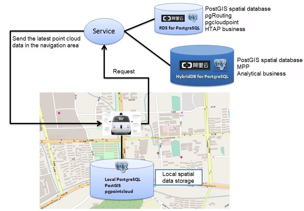
ApsaraDB RDS for PostgreSQL is responsible for online transaction processing (OLTP) and T+0 online analytical processing (OLAP). It is advantageous in the following aspects:
ApsaraDB RDS for PostgreSQL mainly handles online transactions and a small amount of quasi-real-time analysis.
Multi-core parallel computing, JIT, operator reuse, and other features of PostgreSQL allow it to leave other RDBMS databases far behind in terms of OLAP capacity. PostgreSQL 10 also has many enhancements in the aspect of hybrid transaction/analytical processing (HTAP).
PostgreSQL provides rich features.
Complex computing performance can be enhanced by adding additional CPUs.
The storage capacity of ApsaraDB RDS for PostgreSQL can be enhanced using Alibaba Cloud Object Storage Service (OSS) and the OSS_FDW extension, breaking previous storage limitations.
Storage costs: As most of the data that needs to be separated is stored in OSS, users do not need to worry about disaster recovery and backups for this part of the data. Data storage costs in ApsaraDB RDS for PostgreSQL are significantly reduced compared to storing data in databases.
Development costs: Both ApsaraDB RDS for PostgreSQL and AnalyticDB for PostgreSQL support a wide variety of standard SQL APIs, which are also used to access (through table APIs) data stored in OSS. All of these features combined lead to significant reductions in development costs.
Maintenance costs: There is almost no O&M cost when using cloud services.
ApsaraDB RDS for PostgreSQL applies to a wide range of industries, including banking, insurance, securities, IoT, Internet, gaming, astronomy, publishing, e-commerce, traditional enterprises, etc.
AnalyticDB for PostgreSQL uses a massively parallel processing (MPP) architecture and has strong OLAP computing capabilities. Many users with over 100 TB of data are already using AnalyticDB for PostgreSQL in the cloud.
AnalyticDB for PostgreSQL is compatible with PostgreSQL and provides similar features to that of PostgreSQL.
Complex computing performance can be enhanced by adding additional computing nodes.
The storage capacity of AnalyticDB for PostgreSQL can be enhanced by using Alibaba Cloud OSS and the OSS_FDW extension, breaking previous storage limitations.
Storage costs: As most of the data that needs to be separated is stored in OSS, users do not need to worry about disaster recovery and backups for this part of the data. Data storage costs in AnalyticDB for PostgreSQL are greatly reduced compared to storing data in databases.
Development costs: Both ApsaraDB RDS for PostgreSQL and AnalyticDB for PostgreSQL support a wide variety of standard SQL APIs, which are also used to access (through table APIs) data stored in OSS. All of these features combined lead to significant reductions in development costs.
Maintenance costs: There is almost no O&M cost when using cloud services.
AnalyticDB for PostgreSQL applies to a wide range of industries, including banking, insurance, securities, IoT, Internet, gaming, astronomy, publishing, e-commerce, traditional enterprises, etc.
PostgreSQL Best Practices: Supporting 25.1 Billion Parcels Per Day
Technologies Used in Pilotless Driving – Part 2: PostGIS Point Cloud Application
digoal - December 21, 2020
digoal - January 25, 2021
Alibaba Clouder - March 22, 2019
digoal - June 26, 2019
Alibaba Clouder - July 26, 2019
digoal - January 25, 2021
 AnalyticDB for PostgreSQL
An online MPP warehousing service based on the Greenplum Database open source program
Learn More PolarDB for PostgreSQL
Alibaba Cloud PolarDB for PostgreSQL is an in-house relational database service 100% compatible with PostgreSQL and highly compatible with the Oracle syntax.
Learn More AnalyticDB for MySQL
AnalyticDB for MySQL is a real-time data warehousing service that can process petabytes of data with high concurrency and low latency.
Learn More ApsaraDB RDS for PostgreSQL
An on-demand database hosting service for PostgreSQL with automated monitoring, backup and disaster recovery capabilities
Learn MoreMore Posts by digoal