Get Started with Data Structures and Algorithms

What are some common data structures and their basic operations? How are common sorting algorithms implemented? What are the pros and cons of each algorithm? This article aims to address these questions by introducing the basics of sorting algorithms, and by discussing common data structures and common sorting algorithms.

1. Preface

1.1 Why Should We Learn Algorithms and Data Structures?

Solve specific problems.
Optimize program performance.
Learn how to represent problems in computer languages.

1.2 What Business Development Skills Should We Master?

Understand common data structures and algorithms, and can use them flexibly.
Know what data structures and algorithms are required for solving specific problems.

2. Data Structure Basics

2.1 What Is a Data Structure?

A data structure is a data organization, management, and storage format, which is used to efficiently access and modify data.

Data structures are cornerstones of algorithms. By seeing an algorithm as a dancer, the data structure is the stage.

2.2 What Are the Differences Between Physical Structures and Logical Structures?

Physical structures, such as arrays and linked lists, are visible and tangible, just like human flesh, blood, and bones.

Logical structures, such as queues, stacks, trees, and graphs, are invisible and intangible, just like human thoughts and spirits.

2.3 What Are the Differences Between Linear Storage Structures and Non-linear Storage Structures?

In a linear storage structure, elements are one-to-one mapped, such as stacks and queues.
In a non-linear storage structure, each element can be linked to none or multiple elements, such as trees and graphs.

3. Algorithm Basics

3.1 What Is an Algorithm?

In mathematics, an algorithm is used to solve a specific type of problems.
In computers, an algorithm is a series of commands that are used to solve specific computing and logical problems.

3.2 How Can We Measure the Quality of an Algorithm?

Time complexity: by runtime duration
Space complexity: by memory usage

3.3 How Can We Calculate Time Complexities?

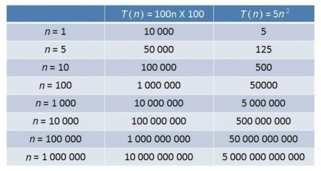
Big O notation (progressive time complexity): simplifies the relative execution time function T(n) of a program into an order of magnitude, such as n, n^2, or logN.

The following rules are used to derive time complexities:

If the runtime is of the constant order of magnitude, the constant is 1.
Only the highest-order term in the time function is retained.
If the highest-order term exists, the coefficient preceding the term is omitted.

Comparison of time complexities: O(1) > O(logn) > O(n) > O(nlogn) > O(n^2)

The following figure shows the number of times each time complexity is run.

3.4 How Can We Calculate Space Complexities?

Constant space O(1): The storage space is fixed in size and is irrelevant to the input scale.

Linear space O(n): The allocated space is a linear collection, and the size of the collection is proportional to the n input scale.

Two-dimensional space O(n^2): The allocated space is a two-dimensional array collection, and the length and width of the collection are proportional to the n input scale.

Recursive space O(logn): Recursion is a special scenario. Although no variables or collections are explicitly declared in recursive code, a memory space is specified to store method call stacks when a program runs on a computer. The memory capacity required by recursion is proportional to the depth of the recursion.

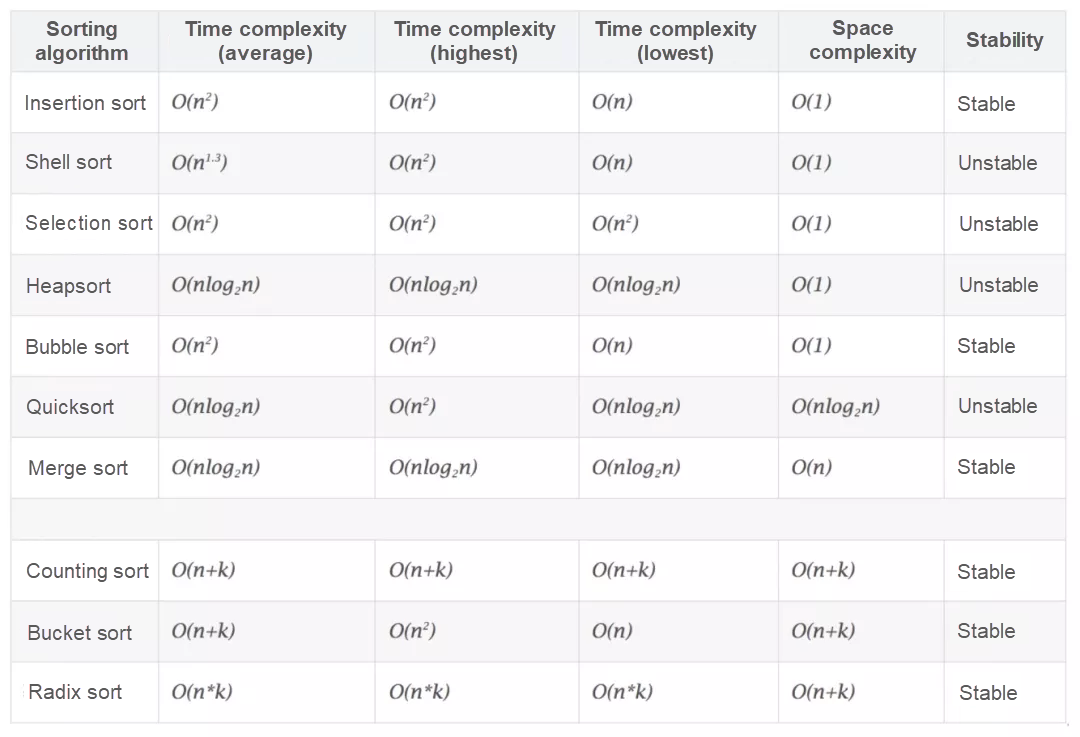
3.5 How Can We Define Algorithm Stability?

Stable: If a is located before b and a is equal to b, a is still located before b after sorting.

Unstable: If a is located before b and a is equal to b, a may be located next to b after sorting.

3.6 What Are Common Algorithms?

Specific algorithms are used to solve specific problems.

String algorithms, such as Brute-Force Matching, Boyer-Moore (BM), Knuth Morris Pratt (KMP), and Trie.
Search algorithms, such as binary search and traversal.
Sorting algorithms, such as bubble sort, comb sort, counting sort, and heap sort.
Retrieval algorithms, such as TF-IDF and PageRank.
Clustering algorithms, such as Expectation Maximisation (EM), K-Means, and K-Medians.
Deep learning algorithms, such as deep belief network (DBN), convolutional neural network (CNN), and generative adversarial network (GAN).
Anomaly detection algorithms, such as K-Nearest Neighbor (KKN) and Local Outlier Factor (LOF).

Among these algorithms, string, search, and sorting algorithms are the most basic ones.

4. Common Data Structures

4.1 Arrays

4.1.1 What Is an Array?

An array is a collection of limited ordered variables of the same type. Each variable in the array is called an element.

4.1.2 What Are Basic Operations on Arrays?

Basic operations on arrays are read O(1), update O(1), insert O(n), delete O(n), and expand O(n).

4.2 Linked Lists

4.2.1 What Is a Linked List?

A linked list is a linear data structure, in which elements are stored at non-contiguous memory locations. It is a data structure consisting of nodes.

Each node in a single linked list contains the data and next fields. The data field stores data of the node, whereas the next field stores the address of the next node.

4.2.2 What Are Basic Operations on Linked Lists?

Basic operations on linked lists are read O(n), update O(1), insert O(1), and delete O(1).

4.2.3 What Are Differences Between Linked Lists and Arrays?

Arrays are suitable for scenarios with more read operations and fewer insert and delete operations.

Linked lists are suitable for scenarios with more insert and delete operations and fewer read operations.

4.3 Stacks

4.3.1 What Is a Stack?

A stack is a linear logical data structure that follows the last in first out (LIFO) principle. The location where the earliest element is stored is called the stack bottom, and the location where the last element is stored is called the stack top.

A stack resembles a pipe with one end blocked and the other open. In contrast, a queue resembles a pipe with both ends open.

4.3.2 How Can We Implement Stacks?

Array implementation

Linked list implementation

4.3.3 What Are Basic Operations on Stacks?

Basic operations on stacks are push O(1) and pop O(1).

4.3.4 What Are Stacks Used For?

Stacks, such as method-call stacks, are used for backtracking.
Stacks are used for breadcrumb navigation on pages.

4.4 Queues

4.4.1 What Is a Queue?

A queue is a linear logical data structure that follows the last in last out (LILO) principle. The exit of a queue is the head of the queue, and the entry of the queue is the tail of the queue.

4.4.2 How Can We Implement Queues?

Array implementation

Linked list implementation

4.4.3 What Are Basic Operations on Queues?

Basic operations on queues are enqueue O(1) and dequeue O(1).

4.4.4 What Are Queues Used For?

Message queues
Multi-thread wait queues
Crawler URL queues

4.5 Hash Tables

4.5.1 What Is a Hash Table?

A hash table is a logical data structure that can map keys to values.

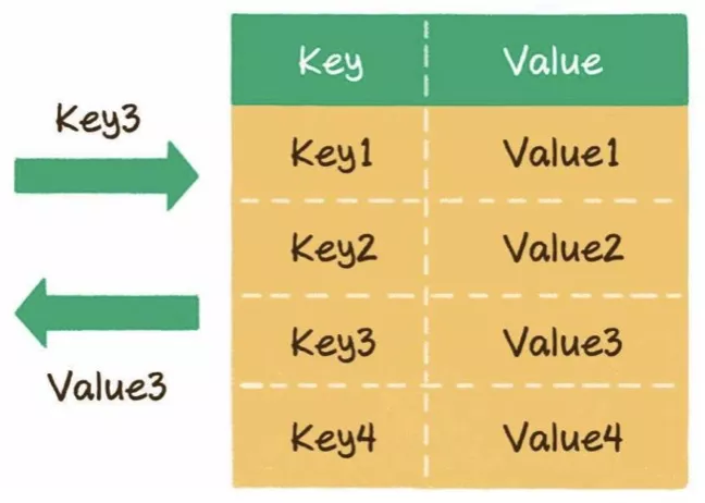
4.5.2 What Are Basic Operations on Hash Tables?

Basic operations on hash tables are read O(1), write O(1), and expand O(n).

4.5.3 What Is a Hash Function?

A hash table is essentially an array that can only be accessed based on subscripts, such as a[0] a[1] a[2] a[3]. Most keys of hash tables are strings.

You can use a hash function to convert a key of string or other types to the index subscript of an array.

Assume that the length of an array is 8.

When the key is 001121, the following information appears:

index = HashCode ("001121") % Array.length = 7

When the key is this, the following information appears:

index = HashCode ("this") % Array.length = 6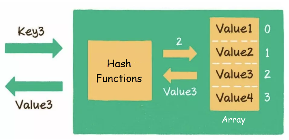

4.5.4 What Are Hash Collisions?

The subscripts obtained by a hash function for different keys may be the same. For example, the array subscripts corresponding to the 002936 and 002947 keys are both 2. This situation is called a hash collision.

4.5.5 What Are Solutions to Hash Collisions?

Linear probing: Threadlocal

Linked list: Hashmap

4.6 Trees

4.6.1 What is a Tree?

A tree is a finite set of n (n ≥ 0) nodes.

When n is 0, the tree is an empty tree. Any tree with at least one node has the following features:

The tree has only one root node.
When n is greater than 1, non-root nodes can be divided into m (m > 0) finite sets that do not intersect with each other. In this case, each set is a subtree of the root node.

4.6.2 What Are Traversal Modes of Trees?

(1) Depth-first search (DFS)

Pre-order traversal: root node, left subtree, and right subtree

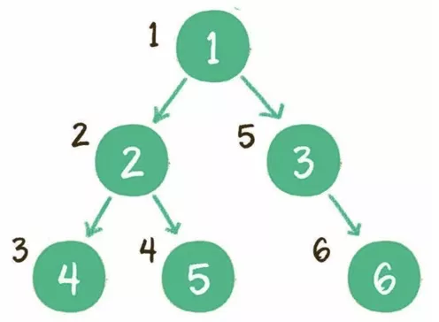
In-order traversal: left subtree, root node, and right subtree

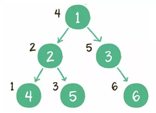
Post-order traversal: left subtree, right subtree, and root node

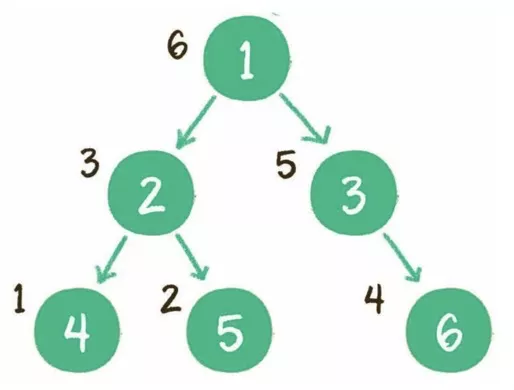
Implementation: recursion or stacks

(2) Breadth-first search (BFS)

Level order traversal: traversal by level

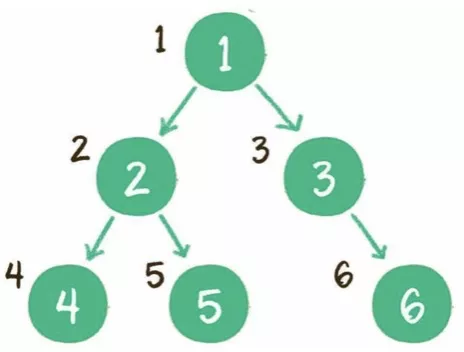
Implementation: queues

4.7 Binary Trees

4.7.1 What Is a Binary Tree?

A binary tree is a special tree. Each node of a binary tree contains up to two child nodes. Specifically, each node of a binary tree can contain 0 to 2 child nodes.

4.7.2 What Is a Full Binary Tree?

Each non-leaf node of a full binary tree contains two child nodes, and all leaf nodes are on the same level.

4.7.3 What Is a Complete Binary Tree?

In a binary tree, all its n nodes are numbered from 1 to n by level. If all the n nodes are in the same positions as the nodes in a full binary tree of the same depth, this tree is a complete binary tree.

4.8 BSTs

4.8.1 What Is a BST?

A binary search tree (BST) is a binary tree that meets the following conditions:

If the left subtree is not empty, values of all nodes in the left subtree are less than the value of the root node.
If the right subtree is not empty, values of all nodes in the right subtree are greater than the value of the root node.
Both the left and right subtrees are BSTs.

4.8.2 What Are BSTs Used For?

Search > Binary search
Sorting > In-order traversal

4.8.3 How Can We Implement a Binary Tree?

Use linked lists.
Use arrays: For sparse binary trees, arrays waste much space.

4.9 Binary Heaps

4.9.1 What Is a Binary Heap?

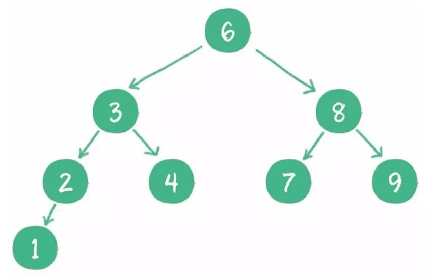
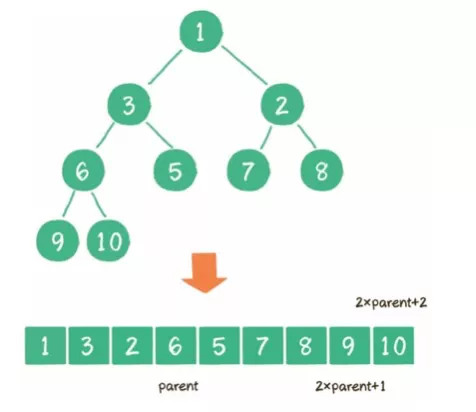
A binary heap is a special complete binary tree that is divided into two types: maximum heaps and minimum heaps.

The value of any parent node of a maximum heap is greater than or equal to the value of each of its left and right child nodes.
The value of any parent node of a minimum heap is less than or equal to the value of each of its left and right child nodes.

4.9.2 What Are Basic Operations on Binary Heaps?

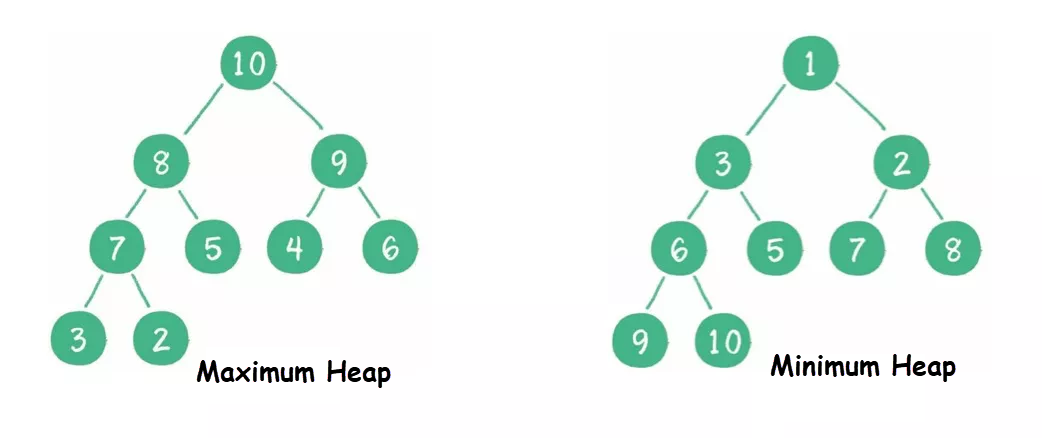
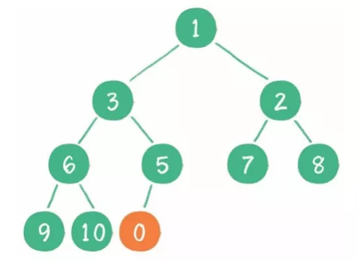
(1) Insert: Insert a node at the end of a binary heap. Then, the nodes rise.

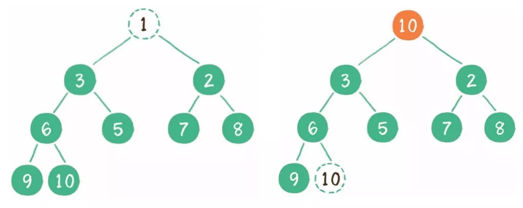
(2) Delete: Delete the head node of a binary heap and move the tail node to the head. Then, the nodes sink.

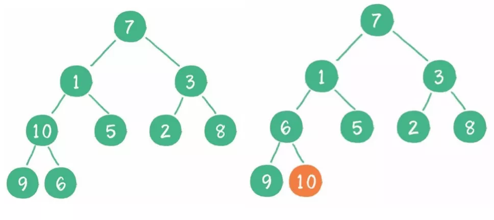
(3) Construct: Construct a binary tree before a binary heap. All non-leaf nodes sink one by one.

4.9.3 How Can We Implement a Binary Heap?

Arrays

5. Common Sorting Algorithms

5.1 Top 10 Classic Sorting Algorithms

5.2 Bubble Sort

(1) Description

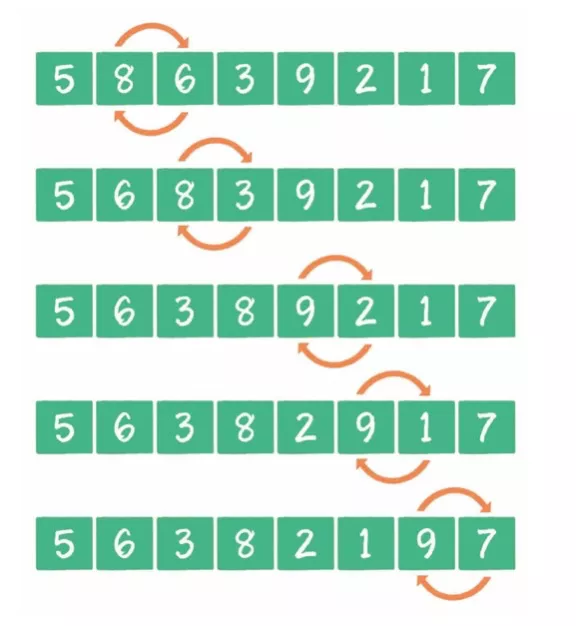
Bubble sort is a simple sorting algorithm. It repeatedly steps through the list, compares two adjacent elements at a time, and swaps them if they are in the wrong order. The pass through the list is repeated until the list is fully sorted. The algorithm, which is a comparison sort, is named for the way smaller elements "bubble" to the top of the list.

(2) Implementation

Compare adjacent elements. If the first element is greater than the second one, the two elements are swapped.
Compare each two adjacent elements in the same way. Then, the last element is the largest.
Repeat the preceding steps on all elements except the last one.
Repeat the preceding steps until the list is fully sorted.

(3) Advantages and disadvantages

Advantages: It is easy to understand and implement.
Disadvantages: The time complexity is O(n^2), and the efficiency is low in the case of many sorting elements.

(4) Scope of application

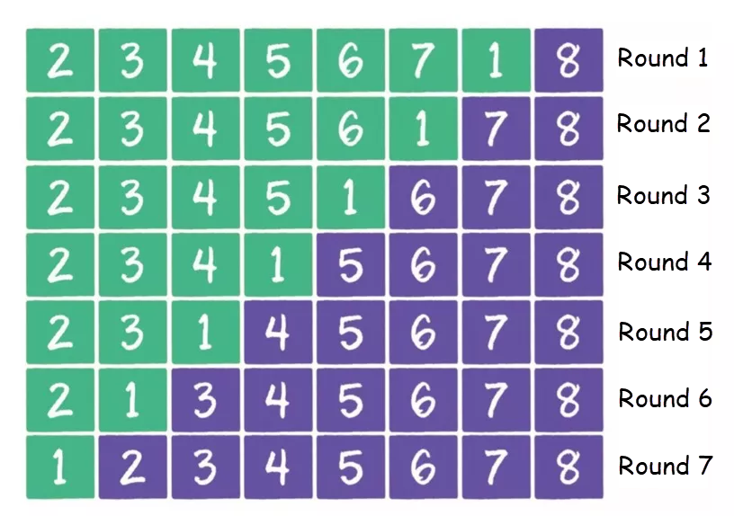
It is applicable to scenarios with a small amount of ordered data.

(5) Scenario optimization

1) Bubble sort continues after the list is sorted

In the current round of sorting, if no elements are swapped, the isSorted value is set to true to exit the major cycle, avoiding unnecessary repetition.

2) The list is partially sorted, but all its elements are traversed in the next round

Record the boundary for sorted elements so that they are not traversed in the next round.

3) All elements must be sorted even if only one of them is out of order

Cocktail sort: extends bubble sort by comparing and swapping elements in two directions.

5.3 Merge Sort

(1) Description

Merge sort is an efficient, merge-based sorting algorithm. This algorithm is a typical divide-and-conquer algorithm. It recursively splits the list into two sublists and then integrates the two sublists while maintaining the element sequence to produce an ordered list.

(2) Implementation

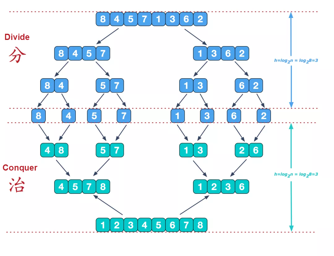
Image source: https://www.cnblogs.com/chengxiao/p/6194356.html

Split an input list of length n into two sublists of length n/2.
Merge-sort elements in the two sublists.
Merge the two sublists into a sorted list.

(3) Advantages and disadvantages

Advantages:

It features good performance and stability, and its time complexity is O(nlogn).
Elements in the list are stably sorted. This algorithm is applicable to more scenarios.

Disadvantages:

Elements are not sorted in place, resulting in a high space complexity.

(4) Scope of application

It is applicable to scenarios where the data volume is large and stable sorting is required.

5.4 Quicksort

(1) Description

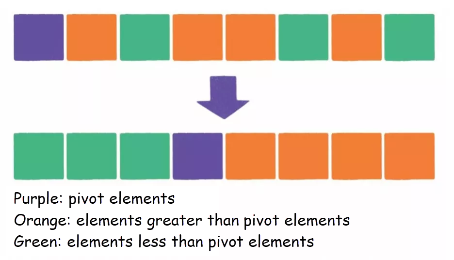
The quicksort algorithm splits a list into a large sublist and a small sublist by using the divide-and-conquer policy. Then, it sorts the two sublists recursively to ensure the eventual sorting of the entire list.

(2) Implementation

Pick an element from a list as the pivot.
Sort the list again. The elements that are less than the pivot are placed in front of it, the elements that are greater than the pivot are placed next to it, and the elements that are equal to the pivot can be in front of or next to it. Then, the pivot is in the middle of the list. This is called a partition operation.
Recursively sort the elements that are less than the pivot and the elements that are greater than the pivot.

(3) Advantages and disadvantages

Advantages:

It features good performance and the lowest time complexity is O(nlogn). In most scenarios, its performance is close to optimal.
Elements in the list are sorted in place. Therefore, the time complexity of this sorting method is lower than that of merge sort.

Disadvantages:

In some scenarios, the worst sorting performance is O(n^2).
Element sorting is unstable.

(4) Scope of application

It is applicable to scenarios where the data volume is large and sorting can be unstable.

(5) Scenario optimization

1) The maximum or minimum element is selected as the pivot each time

Select a non-first element as the pivot.
Select three random numbers and use the middle one as the pivot.

2) The list contains a large amount of repeated data

The data is greater than, less than, or equal to the pivot.

3) Quicksort performance is optimized

Dual pivot quicksort: two pivots, for example, Arrays.sort().

5.5 Heapsort

(1) Description

Heapsort is a sorting algorithm designed based on heaps. A heap is a data structure that approximates a complete binary tree and meets the property requirements of heaps: The key value or index of each child node is always less than (or greater than) that of its parent node.

(2) Implementation

Construct the initial keyword list (R1,R2...Rn) to be sorted into a maximum heap, which is the initial disordered area.
Swap the top element R[1] with the last element R[n] in the heap to generate a new disordered area (R1,R2,...Rn-1) and a new ordered area (Rn), where R[1,2…n-1] <= R[n].
However, the new top element R[1] in the heap may violate the nature of the heap. Therefore, you must adjust the current disordered area (R1,R2,...Rn-1) into a new heap and then swap R[1] with the last element in the disordered area. Then, you can obtain a new disordered area (R1,R2...Rn-2) and a new ordered area (Rn-1,Rn). Repeat this process until the number of elements in the ordered area is n-1. Then, the sorting process ends.

(3) Advantages and disadvantages

Advantages:

It features good performance, and its time complexity is O(nlogn).
The time complexity is relatively constant.
The auxiliary space complexity is O(1).

Disadvantages:

Heap maintenance cost is high when data changes.

(4) Scope of application

It is applicable to scenarios where a large amount of data is input in streaming mode.

(5) Why is quicksort faster than heapsort?

Based on the heapsort process, after the maximum heap is established, the top element is swapped with the last element in the heap, and then the new top element is sunk to the appropriate position. During the sinking process, a large number of almost ineffective comparisons are made because the elements at the bottom are small. Therefore, although the complexity of heapsort and quicksort is both O(NlogN), the constant coefficient of heapsort is greater.

5.6 Counting Sort

(1) Description

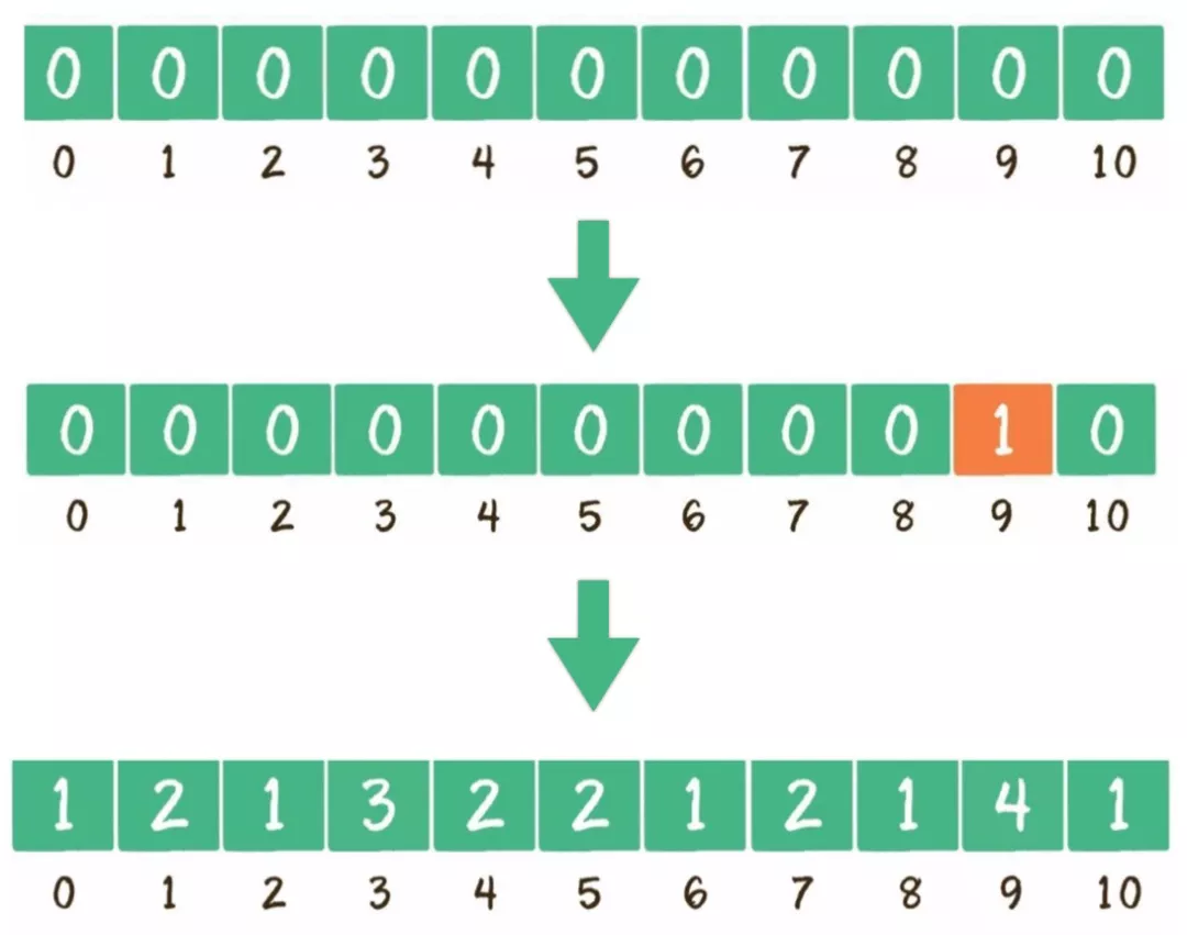
Counting sort is not a comparison-based sorting algorithm. Instead, it aims to convert input data values into keys and store them in extra array space. As a linear sorting algorithm of time complexity, counting sort requires that the input data be integers with specific ranges.

(2) Implementation

Find the element with the largest value in the array to be sorted.
Construct array C with a length of the largest element value plus 1.
Traverse a random disordered array, move each integer to the appropriate position, and increase the subscript of the corresponding array by 1.
Traverse array C and output the subscript values of the array elements. The number of output times for an element is equal to the value of the element.

(3) Advantages and disadvantages

Advantages:

Its performance is much higher than that of a comparison-based algorithm. Its time complexity is O(n+k) where k is the maximum value in the array.
Element sorting is stable.

Disadvantages:

It is applicable to a few scenarios.

(4) Scope of application

The value of each element is an integer. This algorithm is applicable only when the k value in the time complexity is small and the elements concentrate in the list.

(5) Scenario optimization

The number does not start from 0, which may waste space

Use the minimum value in the list as the offset, and the value of (Maximum value – Minimum value + 1) as the length of the list.

5.7 Bucket Sort

(1) Description

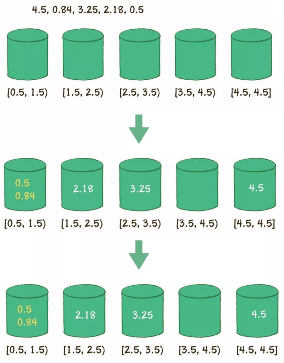
Bucket sort is the upgrade of counting sort. Its efficiency depends on mapping functions. Implementation: Assume that the input data is evenly distributed. Distribute the data into a limited number of buckets, and then sort data in each bucket. You may continue to sort data by using the bucket sort algorithm in a recursive manner or other sorting algorithms.

(2) Implementation

Create buckets and use the following formula to calculate the range: Range = (Maximum value – Minimum value)/(Number of buckets – 1).
Traverse the list and move each element to the appropriate position.
Sort elements in each bucket by using quicksort.
Traverse all buckets and return all elements.

(3) Advantages and disadvantages

Advantages:

The optimal time complexity is O(n), which outperforms a comparison-based sorting algorithm.

Disadvantages:

It is applicable to a few scenarios.
The time complexity is inconstant.

(4) Scope of application

It is applicable to scenarios where data is evenly distributed.

5.8 Performance Comparison

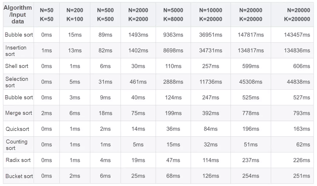
Generate a random list of N numbers in the range from 0 to K. Use various algorithms for sorting and record the time required for each sorting.

References

[1] Cartoon Algorithm: Algorithm Journey of Xiaohui

[2] Algorithms, Fourth Edition

[3] Grokking Algorithms: An Illustrated Guide for Programmers and Other Curious People

[4] For Offers

[5] Top 10 Classic Sorting Algorithms (Demonstrated in Motion Graphs)

[6] Wikipedia

Community

Get Started with Data Structures and Algorithms

1. Preface

1.1 Why Should We Learn Algorithms and Data Structures?

1.2 What Business Development Skills Should We Master?

2. Data Structure Basics

2.1 What Is a Data Structure?

2.2 What Are the Differences Between Physical Structures and Logical Structures?

2.3 What Are the Differences Between Linear Storage Structures and Non-linear Storage Structures?

3. Algorithm Basics

3.1 What Is an Algorithm?

3.2 How Can We Measure the Quality of an Algorithm?

3.3 How Can We Calculate Time Complexities?

3.4 How Can We Calculate Space Complexities?

3.5 How Can We Define Algorithm Stability?

3.6 What Are Common Algorithms?

4. Common Data Structures

4.1 Arrays

4.1.1 What Is an Array?

4.1.2 What Are Basic Operations on Arrays?

4.2 Linked Lists

4.2.1 What Is a Linked List?

4.2.2 What Are Basic Operations on Linked Lists?

4.2.3 What Are Differences Between Linked Lists and Arrays?

4.3 Stacks

4.3.1 What Is a Stack?

4.3.2 How Can We Implement Stacks?

4.3.3 What Are Basic Operations on Stacks?

4.3.4 What Are Stacks Used For?

4.4 Queues

4.4.1 What Is a Queue?

4.4.2 How Can We Implement Queues?

4.4.3 What Are Basic Operations on Queues?

4.4.4 What Are Queues Used For?

4.5 Hash Tables

4.5.1 What Is a Hash Table?

4.5.2 What Are Basic Operations on Hash Tables?

4.5.3 What Is a Hash Function?

4.5.4 What Are Hash Collisions?

4.5.5 What Are Solutions to Hash Collisions?

4.6 Trees

4.6.1 What is a Tree?

4.6.2 What Are Traversal Modes of Trees?

4.7 Binary Trees

4.7.1 What Is a Binary Tree?

4.7.2 What Is a Full Binary Tree?

4.7.3 What Is a Complete Binary Tree?

4.8 BSTs

4.8.1 What Is a BST?

4.8.2 What Are BSTs Used For?

4.8.3 How Can We Implement a Binary Tree?

4.9 Binary Heaps

4.9.1 What Is a Binary Heap?

4.9.2 What Are Basic Operations on Binary Heaps?

4.9.3 How Can We Implement a Binary Heap?

5. Common Sorting Algorithms

5.1 Top 10 Classic Sorting Algorithms

5.2 Bubble Sort

(1) Description

(2) Implementation

(3) Advantages and disadvantages

(4) Scope of application

(5) Scenario optimization

5.3 Merge Sort

(1) Description

(2) Implementation

(3) Advantages and disadvantages

(4) Scope of application

5.4 Quicksort

(1) Description

(2) Implementation

(3) Advantages and disadvantages

(4) Scope of application

(5) Scenario optimization

5.5 Heapsort

(1) Description

(2) Implementation

(3) Advantages and disadvantages

(4) Scope of application

(5) Why is quicksort faster than heapsort?