Using PostgreSQL to Create an Efficient Search Engine

This article goes over how you can use PostgreSQL to create an efficient search engine for full-text searches and other query types including fuzzy and similarity queries.

By Digoal.

Having an efficient and powerful search capability is an important feature of any database. Among search capabilities, a string search is one of the most common and most basic of requirements. There are several types of string searches. They include the following types:

1. Prefix + fuzzy query. For this type, B-tree indexes can be used. Consider the following example expressions:

select * from tbl where col like 'ab%';  
  
or  
  
select * from tbl where col ~ '^ab';

2. Suffix + fuzzy query. For this type, both the reverse(col) expression and B-tree indexes can be used. Again, consider the following examples:

select * from tbl where col like '%ab';  
  
or  
  
select * from tbl where col ~ 'ab$';  
  
Writing  
  
select * from tbl where reverse(col) like 'ba%';  
  
Or 
  
select * from tbl where reverse(col) ~ '^ba';

3. Prefix and/or suffix + fuzzy query. For these, both the pg_trgm and GIN indexes can be used. For more, information, see here.

select * from tbl where col like '%ab%';  
  
or  
  
select * from tbl where col ~ 'ab';

4. Full-text search. For full-text search, the GIN or RUM indexes can be used.

select * from tbl where tsvector_col @@ 'postgres & china | digoal:A' order by ts_rank(tsvector_col, 'postgres & china | digoal:A') limit xx;  

We will discuss the specific syntax later.

5. Regexp query. For this type, both pg_trgm and GIN indexes can be used.

select * from tbl where col ~ '^a[0-9]{1,5}\ +digoal$';

6. Similarity query. pg_trgm and GIN indexes can be used.

select * from tbl order by similarity(col, 'postgre') desc limit 10;

7. Ad Hoc queries, which are queries based on a combination of fields. This category of queries can be implemented by using indexes such as a bloom index, multi-index bitmap scan, or GIN-index bitmap scan. Consider the example below:

select * from tbl where a=? and b=? or c=? and d=? or e between ? and ? and f in (?);

Generally, most databases do not support the acceleration of search queries for the query types 4, 5, 6, and 7 shown above. However, given its powerful capabilities, PostgreSQL can easily support the acceleration of all of the query types given above, including types 4, 5, 6, and 7. This is because, for PostgreSQL, query and write operations are not in conflict with one another, and the relevant indexes can be built in real-time.

Typically with search engines, you do not need to synchronize data before performing queries. As a result, the search engine can only support full-text searches and cannot implement regexp, similarity and prefix/suffix fuzzy queries.

However, with PostgreSQL, you can significantly simplify your overall search engine architecture, reducing the cost of development while also ensuring the capability of real-time data queries.

In the next sections, we will be looking at PostgreSQL-empowered full-text searches, and also the various queries mentioned above. We will consider their core features and also their limitations. Reference links are provided at the end of this article.

Full-text search

The core features of full-text search are: dictionaries, word-breaking syntax, search syntax, sorting algorithms, search efficiency mechanisms, and hit-highlighting, each of which will be discussed below in detail.

These features have been implemented in PostgreSQL, and further extensions to these core features are also supported. For example, dictionaries and sorting algorithms can be extended.

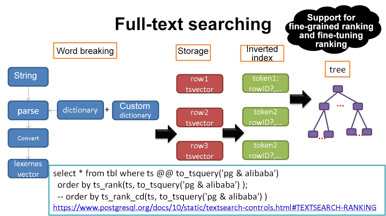
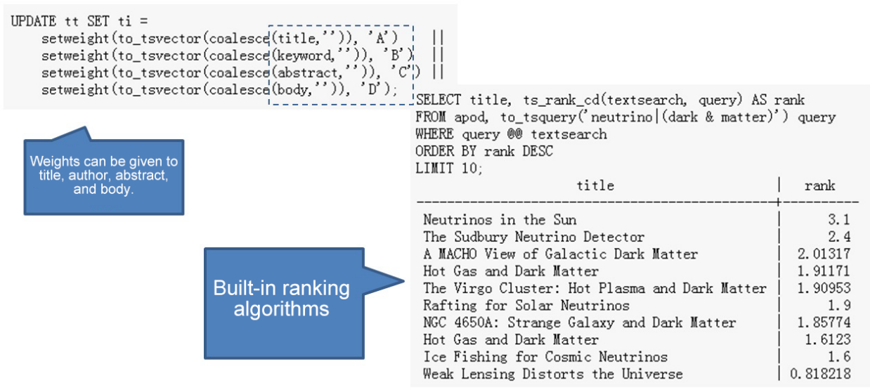
Four document structures are supported. They are the document structures of title, author, abstract, and body. You can specify these structures when generating a tsvector. A tsvector can have multiple document structures.

In a typical ranking algorithm, document structures are used for calculating the weight. For example, you can set a higher weight quantity for a word that pops up in the title than one that pops up in the body.

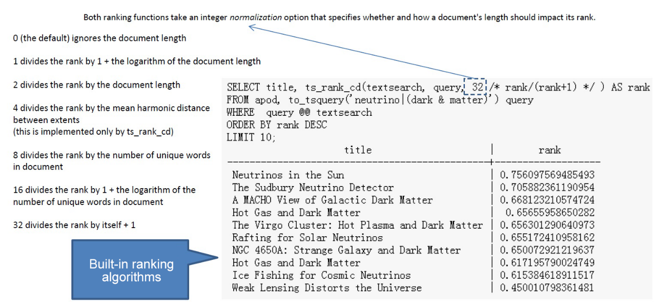
Masking is also supported, mainly so that you can make adjustments for long texts, that is, more specifically so that you can make adjustments to change the output of ranking for these long texts.

You can also set different weights quantities for document structures to adjust the output of ranking.

Dictionaries

One important feature of dictionaries is that the word base allows for word breaking. By default, work breaking is supported and works automatically for English. This functions works pretty well. This is relatively easy to understand-with there being nothing too special for us to say-so we won't go into too much detail here.

However, this is not the case for Chinese as support is not provided for Chinese characters (as well as for other Asian scripts like Japanese, which typically don't add spaces between words). If this is of concern to you-as it has been a concern for Alibaba Cloud's China customers-you can implement extensions based on the text search framework by using Chinese word breaking plug-ins such as the open-source zhparser and jieba. Moreover, modules like pljava and plpython can also be of use for breaking up Chinese words.

Word-Break Syntax

So, now that we've discussed dictionaries and how to add word-break support if you don't have it for your particular language, let's get more in-depth into how word-breaking works at a more microscopic level.

Of the various useful tools out there, there's parser components, which can be used to convert a string into a token. This is very helpful for word-breaking. Of course, parsers can be customized according to your needs. The token types of the default parser that we're using are as follows:

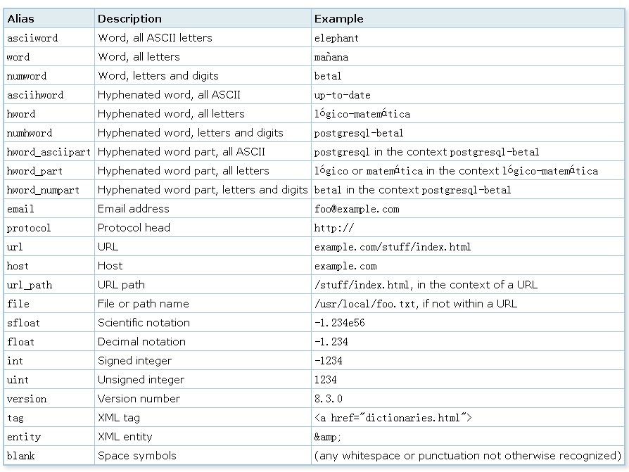
Consider the kind of code that is behind this now:

SELECT alias, description, token FROM ts_debug('http://example.com/stuff/index.html');  
  alias   |  description  |            token               
----------+---------------+------------------------------  
 protocol | Protocol head | http://  
 url      | URL           | example.com/stuff/index.html  
 host     | Host          | example.com  
 url_path | URL path      | /stuff/index.html

To learn more about related syntax, check out this page.

Next, another thing you can do is convert tokens into lexemes with text search configuration and dictionaries. For example, consider this, you can create a synonym dictionary:

postgres        pgsql  
postgresql      pgsql  
postgre pgsql  
gogle   googl  
indices index*

Next, following this, you can use this dictionary to convert tokens into lexemes. Note that a tsvector also stores lexemes rather than original tokens. Consider the following:

mydb=# CREATE TEXT SEARCH DICTIONARY syn (template=synonym, synonyms='synonym_sample');  
mydb=# SELECT ts_lexize('syn','indices');  
 ts_lexize  
-----------  
 {index}  
(1 row)  
  
mydb=# CREATE TEXT SEARCH CONFIGURATION tst (copy=simple);  
mydb=# ALTER TEXT SEARCH CONFIGURATION tst ALTER MAPPING FOR asciiword WITH syn;  
mydb=# SELECT to_tsvector('tst','indices');  
 to_tsvector  
-------------  
 'index':1  
(1 row)  
  
mydb=# SELECT to_tsquery('tst','indices');  
 to_tsquery  
------------  
 'index':*  
(1 row)  
  
mydb=# SELECT 'indexes are very useful'::tsvector;  
            tsvector               
---------------------------------  
 'are' 'indexes' 'useful' 'very'  
(1 row)  
  
mydb=# SELECT 'indexes are very useful'::tsvector @@ to_tsquery('tst','indices');  
 ?column?  
----------  
 t  
(1 row)

To learn more about the syntax used to create a text dictionary, visit this page.

Next, you can also store lexemes in a tsvector. For this, the text search configuration decides the content to be stored. Then, during the conversion process, tokens converted by the parser will be matched to entries in the dictionaries specified by the configuration, and corresponding lexemes in the dictionaries will be stored.

ALTER TEXT SEARCH CONFIGURATION tsconfig name  
    ADD MAPPING FOR token type 1 WITH dictionary 1, dictionary 2, dictionary 3;  
  
If the tsconfig is used to convert the text into a tsvector, Token Type 1 will first match against Dictionary 1. If they match successfully, lexemes in Dictionary 1 will be stored. If they do not match, the search proceeds to Dictionary 2.

To learn more about the syntax used to create text search configuration, see this page.the specific syntax used to create a text search template, check out this page.

Next, there's Control parameters. A parser will usually contain a few of these, for example, to control whether a single character or two characters will be returned or not.

And last, of course, there's also document structures, which are such things as the title, author, abstract, and body. They are usually represented by A, B, C, and D, respectively.

Search syntax

When it comes to search syntax, there's some important concepts to cover. One of these is that a tsquery stores lexemes that are to be searched for, and supports the operators AND, OR, NOT, and FOLLOWED BY. For example, to_tsquery creates a tsquery value from query text, which must consist ofsingle tokens separated by the tsquery operators:

& (AND), | (OR), ! (NOT), and <-> (FOLLOWED BY) and <?> (How far away is it?),

You can group operators using parentheses. That is, the input to to_tsquery must already follow the general rules for tsquery input.

The difference is that, while basic tsquery input takes the tokens as they are originally inputted, to_tsquery normalizes each token into a lexeme using the configurations you specified or the default configurations and also discards any tokens that are stop words according to the configuration. For example, consider the following:

c There are two positions both of which can be used when matching distances.
postgres=# select to_tsvector('a b c c');
     to_tsvector     
---------------------
 'a':1 'b':2 'c':3,4
(1 row)

Adjacent
postgres=# select to_tsvector('a b c c') @@ to_tsquery('a <-> b');
 ?column? 
----------
 t
(1 row)

Adjacent, means that, when the positions are subtracted by each other, they are equal to one. 
postgres=# select to_tsvector('a b c c') @@ to_tsquery('a <1> b');
 ?column? 
----------
 t
(1 row)

When the distance is 2, then, when the positions are subtracted by each other, they are equal to 2.
postgres=# select to_tsvector('a b c c') @@ to_tsquery('a <2> c');
 ?column? 
----------
 t
(1 row)

When the distance is 3, then, when the positions are subtracted by each other, they are equal to 3.
postgres=# select to_tsvector('a b c c') @@ to_tsquery('a <3> c');
 ?column? 
----------
 t
(1 row)

When the distance is 2, then, when the positions are subtracted by each other, they are equal to 2.
postgres=# select to_tsvector('a b c c') @@ to_tsquery('a <2> b');
 ?column? 
----------
 f
(1 row)

Next, document structures are supported. For this, the syntax is as follows. As with basic tsquery input, weights can be attached to each lexeme to restrict it to match only tsvector lexemes of those weights. For example, consider the following:

SELECT to_tsquery('english', 'Fat | Rats:AB');  
    to_tsquery      
------------------  
 'fat' | 'rat':AB

Next, prefix matching is also supported. Consider the following example. Notice that in this below example, * is attached to a lexeme for prefix matching purposes:

SELECT to_tsquery('supern:*A & star:A*B');  
        to_tsquery          
--------------------------  
 'supern':*A & 'star':*AB

Next, features such as nested thesaurus dictionaries and automatic translation are also supported. Consider the following example. to_tsquery can also accept single-quoted phrases. This is useful because the configuration can include a thesaurus dictionary that may be triggered by such phrases. In the example below, a thesaurus contains the rule supernovae stars : sn:.

SELECT to_tsquery('''supernovae stars'' & !crab');  
  to_tsquery  
---------------  
 'sn' & !'crab'

Next, it is important to note that the search operator is @@, as you can see in the example below:

select * from tbl where $tsvector_col @@ $tsquery;

Sorting Algorithms

When it comes down to sorting algorithms, full-text searching usually involves two aspects: matching and ranking.

On the ranking side of things, PostgreSQL has several built-in ranking algorithms, such as this one: src/backend/utils/adt/tsrank.c. As for this, it's important to understand both ts_rank and ts_rank_cd. PostgreSQL provides both of these two predefined ranking functions, which take into account lexical and structural information as well as proximity information. That is, these predefined ranking function consider how often the query terms appear in a document, how close they appear in the document, and in which part of the document they occur (and also whether this part of the document relatively speaking is of a high weight or not).

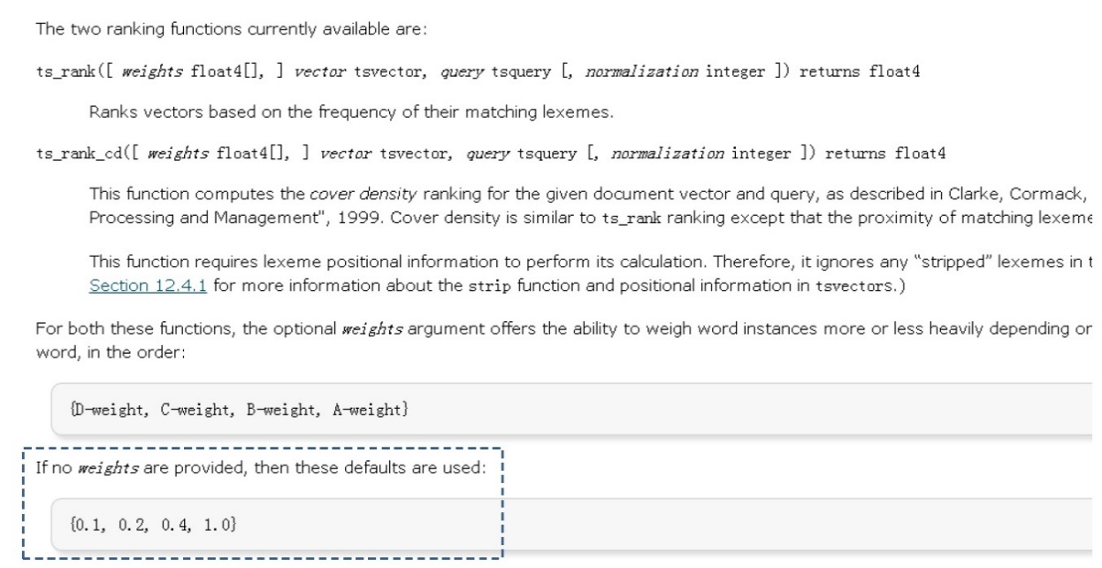
You can write your own ranking functions with these two predefined ranking functions, and combine their results with additional factors to fit your specific needs. The two ranking functions currently available are ts_rank and ts_rank_cd.

ts_rank([ weights float4[], ] vector tsvector, query tsquery [, normalization integer ]) returns float4

This first function ranks vectors based on the frequency of their matching lexemes.

ts_rank_cd([ weights float4[], ] vector tsvector, query tsquery [, normalization integer ]) returns float4

Next, ts_rank_cd is used for the cover density ranking. As described in Clarke, Cormack, and Tudhope's "Relevance Ranking for One to Three Term Queries" in the journal "Information Processing and Management", 1999, cover density ranking is similar to ts_rank ranking except that the proximity of the matching lexemes which each other is taken into consideration.

Both of the preceding ranking functions support adding the weight(s) of document structures. Furthermore, you can fine-tune these weights, and can enter the weights as array parameters. If no weights are provided, default weights will be used.

For both these functions, with the flexibility to set weights you have the ability to weigh word instances more or less heavily depending on how they are labeled. The weight arrays specify how heavily to weigh each category of word, in the following order:

{D-weight, C-weight, B-weight, A-weight}

If no weights are provided, then these default weight configurations are used:

{0.1, 0.2, 0.4, 1.0}

Next, mask parameters are supported to process long parameters. Because a longer document has a greater chance of containing a query term, it is reasonable to take into account document size.

For example, consider this: a hundred-word document with five instances of a search word is probably much more relevant than a thousand-word document with five instances of the word. Both ranking functions take an integer normalization option that specifies whether and how a document's length should impact its rank. The integer option controls several behaviors, so it's like a bit mask: you can specify one or more behaviors using | (for example, 2|4).

Below is an mask example:

0 (the default) ignores the document length  
  
1 divides the rank by 1 + the logarithm of the document length  
  
2 divides the rank by the document length  
  
4 divides the rank by the mean harmonic distance between extents (this is implemented only by ts_rank_cd)  
  
8 divides the rank by the number of unique words in document  
  
16 divides the rank by 1 + the logarithm of the number of unique words in document  
  
32 divides the rank by itself + 1

If more than one flag bit is specified, the transformations are applied in the order listed. Next, below is another example where only the ten highest-ranked matches are selected:

SELECT title, ts_rank_cd(textsearch, query) AS rank  
FROM apod, to_tsquery('neutrino|(dark & matter)') query  
WHERE query @@ textsearch  
ORDER BY rank DESC  
LIMIT 10;  
                     title                     |   rank  
-----------------------------------------------+----------  
 Neutrinos in the Sun                          |      3.1  
 The Sudbury Neutrino Detector                 |      2.4  
 A MACHO View of Galactic Dark Matter          |  2.01317  
 Hot Gas and Dark Matter                       |  1.91171  
 The Virgo Cluster: Hot Plasma and Dark Matter |  1.90953  
 Rafting for Solar Neutrinos                   |      1.9  
 NGC 4650A: Strange Galaxy and Dark Matter     |  1.85774  
 Hot Gas and Dark Matter                       |   1.6123  
 Ice Fishing for Cosmic Neutrinos              |      1.6  
 Weak Lensing Distorts the Universe            | 0.818218

Then, here's the same example using normalized ranking:

SELECT title, ts_rank_cd(textsearch, query, 32 /* rank/(rank+1) */ ) AS rank  
FROM apod, to_tsquery('neutrino|(dark & matter)') query  
WHERE  query @@ textsearch  
ORDER BY rank DESC  
LIMIT 10;  
                     title                     |        rank  
-----------------------------------------------+-------------------  
 Neutrinos in the Sun                          | 0.756097569485493  
 The Sudbury Neutrino Detector                 | 0.705882361190954  
 A MACHO View of Galactic Dark Matter          | 0.668123210574724  
 Hot Gas and Dark Matter                       |  0.65655958650282  
 The Virgo Cluster: Hot Plasma and Dark Matter | 0.656301290640973  
 Rafting for Solar Neutrinos                   | 0.655172410958162  
 NGC 4650A: Strange Galaxy and Dark Matter     | 0.650072921219637  
 Hot Gas and Dark Matter                       | 0.617195790024749  
 Ice Fishing for Cosmic Neutrinos              | 0.615384618911517  
 Weak Lensing Distorts the Universe            | 0.450010798361481

Ranking can be expensive since it requires consulting the tsvector of each matching document, which can be limited, or bound, by your I/O restrictions, and therefore it may be slow as a result. Unfortunately, this is almost impossible to avoid because practical queries often result in large numbers of matches.

Search Efficiency Mechanisms

When it comes to efficiency, there are several mechanisms to improve the overall system. First there is the write efficiency mechanism, which randomly obtains 64 words from a lexicon of 5 million words and makes up a string that is consisting of the 64 words. GIN indexes for full text searches are included. Next, there is also the query efficiency mechanism, which performs a full-text search on just 100 million text records.

Special features

HTML Highlighting Feature

Of the special features, first there is the HTML highlighting feature, which can highlight matching text. It is as follows:

ts_headline([ config regconfig, ] document text, query tsquery [, options text ]) returns text

An example output is as follows:

SELECT ts_headline('english',  
  'The most common type of search  
is to find all documents containing given query terms  
and return them in order of their similarity to the  
query.',  
  to_tsquery('query & similarity'));  
  
                        ts_headline                           
------------------------------------------------------------  
 containing given <b>query</b> terms  
 and return them in order of their <b>similarity</b> to the  
 <b>query</b>.  
  
SELECT ts_headline('english',  
  'The most common type of search  
is to find all documents containing given query terms  
and return them in order of their similarity to the  
query.',  
  to_tsquery('query & similarity'),  
  'StartSel = <, StopSel = >');  
                      ts_headline                        
-------------------------------------------------------  
 containing given <query> terms  
 and return them in order of their <similarity> to the  
 <query>.

Generate Document Statistics Feature

Next, there is the generate document statistics feature. How this feature works is that the sqlquery returns a tsvector column and counts which lexemes are included in this column. Furthermore, it also counts how many texts each lexeme appears and how many times each lexeme totally appears. An example of this one is as follows:

ts_stat(sqlquery text, [ weights text, ]  
        OUT word text, OUT ndoc integer,  
        OUT nentry integer) returns setof record

It returns the following values:

word text - the value of a lexeme  
  
ndoc integer - number of documents (tsvectors) the word occurred in  
  
nentry integer - total number of occurrences of the word

Consider this following example. This example is used to find the ten most frequent words in a document collection:

SELECT * FROM ts_stat('SELECT vector FROM apod')  
ORDER BY nentry DESC, ndoc DESC, word  
LIMIT 10;

This one is similar but is used for counting only word occurrences with a weight of A or B:

SELECT * FROM ts_stat('SELECT vector FROM apod', 'ab')  
ORDER BY nentry DESC, ndoc DESC, word  
LIMIT 10;

Setting Document Structure Feature

Next, there's the setting document structure feature, which set which document structure a tsvector belongs to, which would, of course, be one of the following structures: title, author, abstract, or body. Consider the following example:

1、  
setweight(vector tsvector, weight "char")      
  
assign weight to each element of vector      
  
setweight('fat:2,4 cat:3 rat:5B'::tsvector, 'A')      
'cat':3A 'fat':2A,4A 'rat':5A  
  
2、  
setweight(vector tsvector, weight "char", lexemes text[])  
  
assign weight to elements of vector that are listed in lexemes      
  
setweight('fat:2,4 cat:3 rat:5B'::tsvector, 'A', '{cat,rat}')      
'cat':3A 'fat':2,4 'rat':5A

Debugging Text Feature

Last, there is the special feature for debugging text. This figure can be used to debug a text for tokens. See this document for more information about this feature. Consider the following example.

ts_debug([ config regconfig, ] document text,  
         OUT alias text,  
         OUT description text,  
         OUT token text,  
         OUT dictionaries regdictionary[],  
         OUT dictionary regdictionary,  
         OUT lexemes text[])  
         returns setof record  
alias text - short name of the token type  
  
description text - description of the token type  
  
token text - text of the token  
  
dictionaries regdictionary[] - the dictionaries selected by the configuration for this token type  
  
dictionary regdictionary - the dictionary that recognized the token, or NULL if none did  
  
lexemes text[] - the lexeme(s) produced by the dictionary that recognized the token,   
or NULL if none did; an empty array ({}) means it was recognized as a stop word

Then, for Debug lexemes, ts_lexize can be used to judge if a token has matching lexemes in a certain dictionary.

ts_lexize(dict regdictionary, token text) returns text[]

For example:

SELECT ts_lexize('english_stem', 'stars');  
 ts_lexize  
-----------  
 {star}  
  
SELECT ts_lexize('english_stem', 'a');  
 ts_lexize  
-----------  
 {}

Limitations

Now that we have looked at the core features of full-text search, in addition to some additional special features, now it's time to consider some of the limitations of this query type. First, among other limitations of this query type, there is the fact that the length of each lexeme must be less than 2K bytes. Furthermore, the length of a tsvector (lexemes + positions) must be less than 1 megabyte. Consider the following error related to this limit:

postgres=# select length(to_tsvector(string_agg(md5(random()::text), ' '))) from generate_series(1,100000);  
ERROR:  54000: string is too long for tsvector (3624424 bytes, max 1048575 bytes)  
LOCATION:  make_tsvector, to_tsany.c:185

In a tsvector, the number of lexemes must be less than 2^64 (which happens to be 18446744073709551616, if you do the math).

Another limitation is that the position values in tsvector must be greater than 0 and no more than 16,383. Similarly, the match distance in a (FOLLOWED BY) tsquery operator cannot be more than 16,384. And another limit is that no more than 256 positions per lexeme. Following this, the number of nodes (lexemes + operators) in a tsquery must be less than 32,768.

In general, if you find yourself to be limited by these limitation-hitting a brick wall when conducting full-text search-you'll need to use more fields to compensate.

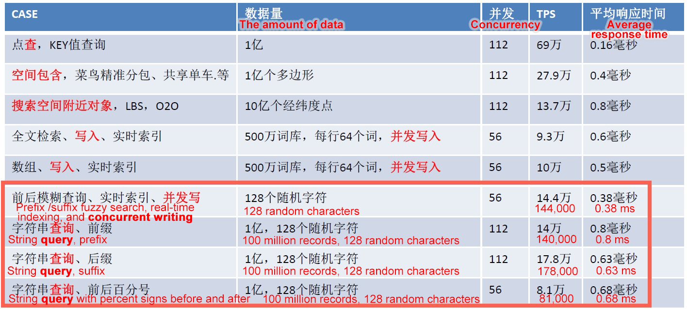
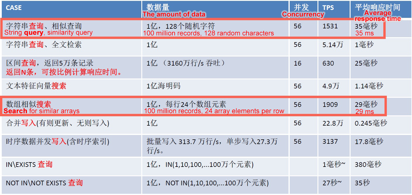
Other Query Types: Fuzzy, Regexp, and Similarity queries

Fuzzy queries, regexp queries, and similarity queries are all more or less related to text matching. In PostgreSQL, GIN and pg_trgm is provided to speed up these three types of searches by using indexes.

The performance of these queries is as follows:

Ad Hoc Searches

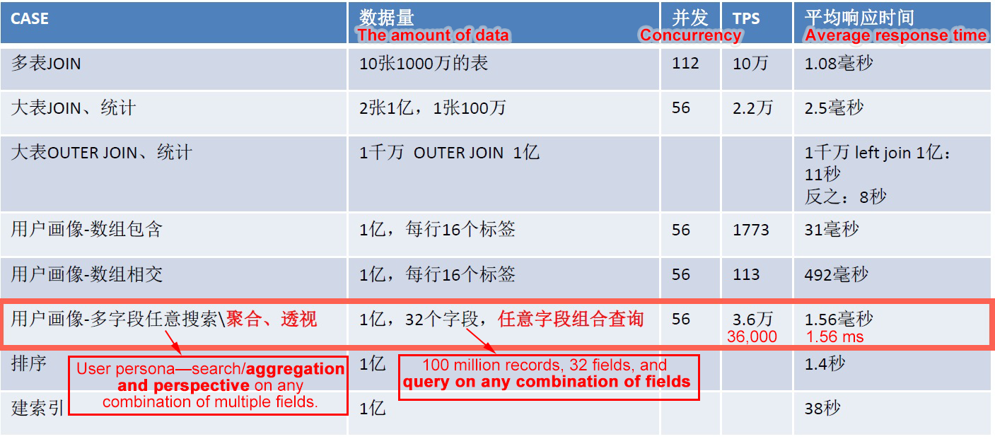
Ad Hoc searches refer to searches that rely on a combination of several different fields. For example, if a table has N columns and all the N columns may be the query criteria. Therefore, the number of all possible combinations is N!. PostgreSQL provides several methods to implement efficient searching in this kind of scenarios:

Partition tables, which can implement convergence when a search is based on several various fields.
Bloom filter indexes, which support equivalent searches in any combination of fields. Similar to these are lossy filters.
GIN multi-column composite indexes and BITMAP scans. For these, searching based on any combinations is supported, and filtering can be implemented at the block level.
Multiple single-column indexes and BITMAP scans. For these, databases are automatically optimized, then, the option of whether to choose index scans or bitmap scans is determined based on the cost evaluation. Next, searching based on any combination of fields is supported. Filtering at the block level is also supported.

The performance of these various Ad Hoc searches is as follows:

References

1. Full-text search
https://www.postgresql.org/docs/10/static/textsearch.html
https://www.postgresql.org/docs/10/static/textsearch-controls.html#TEXTSEARCH-PARSING-QUERIES

2. Fuzzy query, regexp query, and similarity query
https://www.postgresql.org/docs/10/static/pgtrgm.html

3. Ad Hoc query
https://www.postgresql.org/docs/10/static/indexes-bitmap-scans.html
https://www.postgresql.org/docs/10/static/bloom.html
https://www.postgresql.org/docs/10/static/gin.html

4.
Starting from the difficult fuzzy search-principles and technical background of the GIN, GiST, SP-GiST, RUM indexes of PostgreSQL
Full-text search with PostgreSQL is way too fast-RUM index interface (Pandora box)
PostgreSQL supports efficient full-table query, full-field query, and fuzzy query in milliseconds, bringing significant advantages on search engines

Community

Using PostgreSQL to Create an Efficient Search Engine

Full-text search

Dictionaries

Word-Break Syntax

Search syntax

Sorting Algorithms

Search Efficiency Mechanisms

Special features

HTML Highlighting Feature

Generate Document Statistics Feature

Setting Document Structure Feature

Debugging Text Feature

Limitations

Other Query Types: Fuzzy, Regexp, and Similarity queries

Ad Hoc Searches

References

Read previous post:

Read next post:

digoal

You may also like

Comments

digoal

Related Products

OpenSearch

Image Search

PolarDB for PostgreSQL

Database Overview