In May 2026, the Google Cloud DORA team published ROI of AI-Assisted Software Development. Unlike DORA Accelerate State of DevOps Report 2025 from the previous year, which focused on individual adoption rates, this report directly addresses an organization-level issue:
"The question is no longer whether AI-assisted development works — it's how to prove it to the business."
The report provides a group of model data. Taking an engineering team of 500 staffs as an example, the annual investment in AI tools is approximately $8.4 million, the expected return is $11.6 million, and the first-year ROI is approximately 39%. However, this return is not automatically realized. DORA explicitly points out that the improvement in coding speed does not automatically result in conversion into organization output:
"Initial gains in coding speed are promising, but they don't automatically translate to the bottom line."
The report introduces the concept of the J-Curve (a curve that first drops and then rises) to explain the mechanism. The team will experience a productivity decline period in the early stage of adopting AI tools. Workflow adaptation, habit switch, and prompt tuning are all learning costs. Only after the team passes this trough and reinvests the recovered capacity to reduce rework instead of directly cutting manpower, will the ROI be realized in the later segment of the curve. At the same time, DORA continues the core judgment of the 2025 report:
"AI is an amplifier, not a transformer. It magnifies strengths and dysfunctions."
Data shows that AI can bring an efficiency gain of 35% to 40% on greenfield projects, but less than 10% on legacy code. Such a huge difference means that the return curves of different teams within the same company may be completely different. An organization without event-level measure capabilities cannot even judge where its own J-Curve has reached.
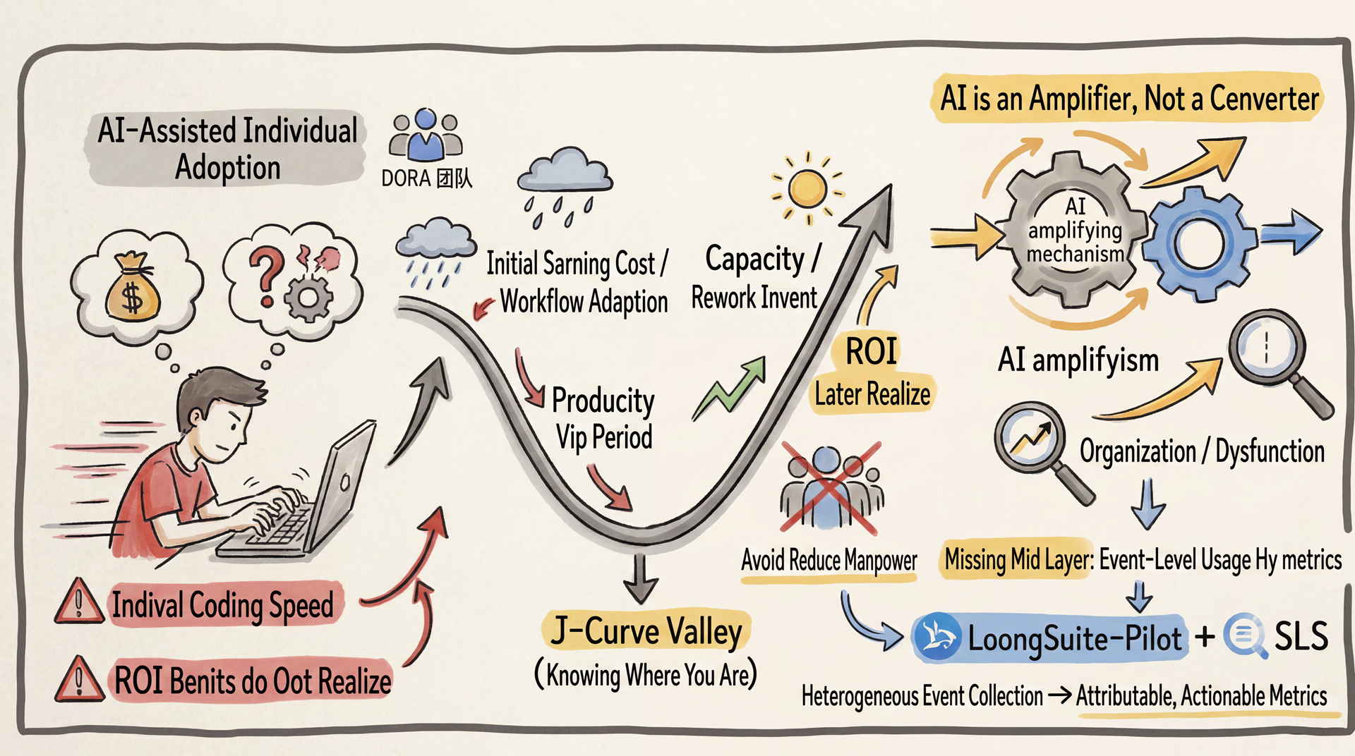
This is exactly the dilemma of most current research and development organizations: they only have two classes of data in hand. One is the self-reported satisfaction questionnaire of individuals (subjective and untraceable), and the other is the aggregation KPI of the CI/CD pipeline (which tells you what, but does not explain why). What is truly missing is the middle layer: the event-level AI coding usage behavior measure that can drill down to the Agent, model, skill, or department. This allows the organization to accurately answer where the J-Curve has reached, which teams are already in the later segment of the curve, and which are still in the trough.
The LoongSuite-Pilot × Alibaba Cloud Simple Log Service (SLS) integration introduced in this topic is exactly the engineering implementation of this measure layer. LoongSuite-Pilot uniformly collects the event streams of heterogeneous Agents according to the LoongSuite GenAI semantics specification (an extension specification launched by Alibaba Cloud based on the OpenTelemetry GenAI semantic conventions). The SLS dashboard interprets the events into organization-level measures that can be used to drill down, perform attribution, and take actions.
Before you build the measure dashboard, you can first solve the problem of where the data comes from.
What we choose to measure is not how many lines of code are committed or how many pull requests (PRs) are merged, but the usage behavior of the AI coding Agent itself: who uses which Agent, which model is selected, how many tokens are consumed, and which tools and skills are invoked.
The data model adopts the classic separation design of the fact table and the dimension table. The two tables are associated through user.id and work_no. The separation of the fact table and the dimension table allows the measure layer to flexibly superimpose organization dimensions through JOIN, without the need to embed organization information during event reporting.
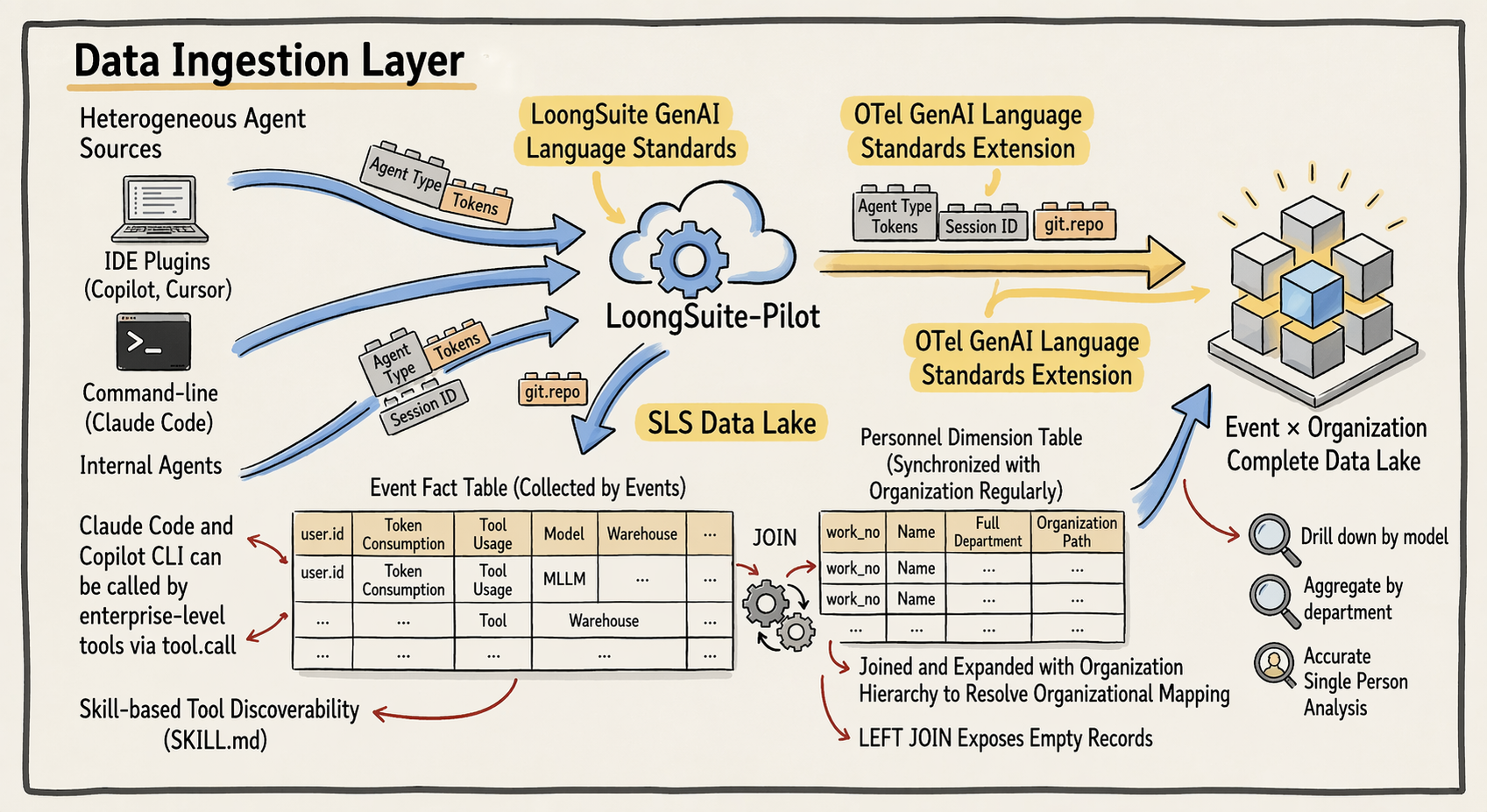
The fact table is the core data source of the entire measure dashboard. Each record corresponds to one Agent invoke event. The core fields include:
User identifier: user.id.
Session: gen_ai.session.id.
Agent/Provider/Model: gen_ai.agent.type, gen_ai.provider.name, gen_ai.request.model, and gen_ai.response.model.
Token consumption: gen_ai.usage.input_tokens, gen_ai.usage.output_tokens, and gen_ai.usage.total_tokens.
Tool calling: gen_ai.tool.name, gen_ai.tool.call.arguments.file_path, and event.name.
These fields align with the LoongSuite GenAI semantics specification. OpenTelemetry GenAI semantic conventions are recognized by the industry as a starting point. However, community standards naturally need to balance broad applicability and long-term stability, and are currently still in the development status. In actual business, the invocation chain of AI Agents is often much more complex than "single user × single model." A request may span the collaborative invocation of multiple agents.
The LoongSuite GenAI semantics specification is exactly an extension specification derived from a large number of practical scenarios based on the OpenTelemetry community standards. The specification is officially open-source now, and the optimization capabilities will be gradually contributed to the community upstream in the future. The direct benefit of aligning with this specification is that the reporting metrics of Claude Code, Copilot, Cursor, Qoder, and various internal Agents are naturally consistent. You do not need to perform field reconciliation afterward.
These events are uniformly collected through LoongSuite-Pilot. LoongSuite-Pilot does not distinguish between agent sources and integrated development environment (IDE) forms. Whether it is Claude Code in the command line form or Copilot or Cursor in the IDE plugin form, they all fall into the same fact table. The collection granularity is at the event level. Each agent invocation, each tool call, and each token consumption are reported as independent events, rather than being reported after being aggregated by session.
The event-level granularity brings three engineering values:
First, comparability of heterogeneous agents: The statistics metric of the same token under Claude Code and Copilot is completely consistent. Cross-tool comparison and aggregation do not require any metric conversion.
Second, session-level traceability: By drilling from gen_ai.session.id to a single tool.call, troubleshooting can be accurate to "what parameters were passed in the third tool calling in this session," rather than stopping at "this person had a high token consumption last week."
Third, observability of skills and tools:gen_ai.tool.call.arguments.file_path associates the tool calling with the specific SKILL.md file path, making "whether the skills accumulated by the team are really used" a quantifiable problem.
The event stream resolves "what happened," and the personnel dimension table resolves "who is doing it." The user identifier in an event is mapped to the organization topology, so that the measure can drill down by department, team, and personnel. The dimension table is periodically synchronized to SLS. The core fields are work_no (employee ID), show_name (name), and dept_name (full department path, such as Technology R&D Department - Engineering Platform Department – Data Service group).
Why must the organization relationship be integrated as an independent dimension table, rather than injecting department information into the event when the event is reported? There are three reasons:
First, decoupling. The personnel dimension table is continuously updated with organization adjustments, but once an event is reported, it should not be retroactively modified. Only when the dimension table is independent can you "view historical data based on the latest organization structure."
Second, LEFT JOIN exposes blanks. For employees who have records in the dimension table but no records in the event table, you can directly list the people who are "registered but not reported" through LEFT JOIN + WHERE user_id IS NULL. This list of "registered but not reported" people can often drive implementation better than all cool charts.
Third, level splitting is completed at one time. The department path is split by level into three layers: tier-1 department, tier-2 department, and team. All downstream charts only need to JOIN the dimension table to obtain the complete organization dimension. You do not need to repeat the splitting logic for each graph.
The core questions answered by the data integration layer boil down to three: what to collect (LoongSuite GenAI semantics events), how to collect (uniform collection by LoongSuite-Pilot), and who to associate with (personnel dimension table). After the three steps are completed, SLS has a complete data foundation of "event × organization."
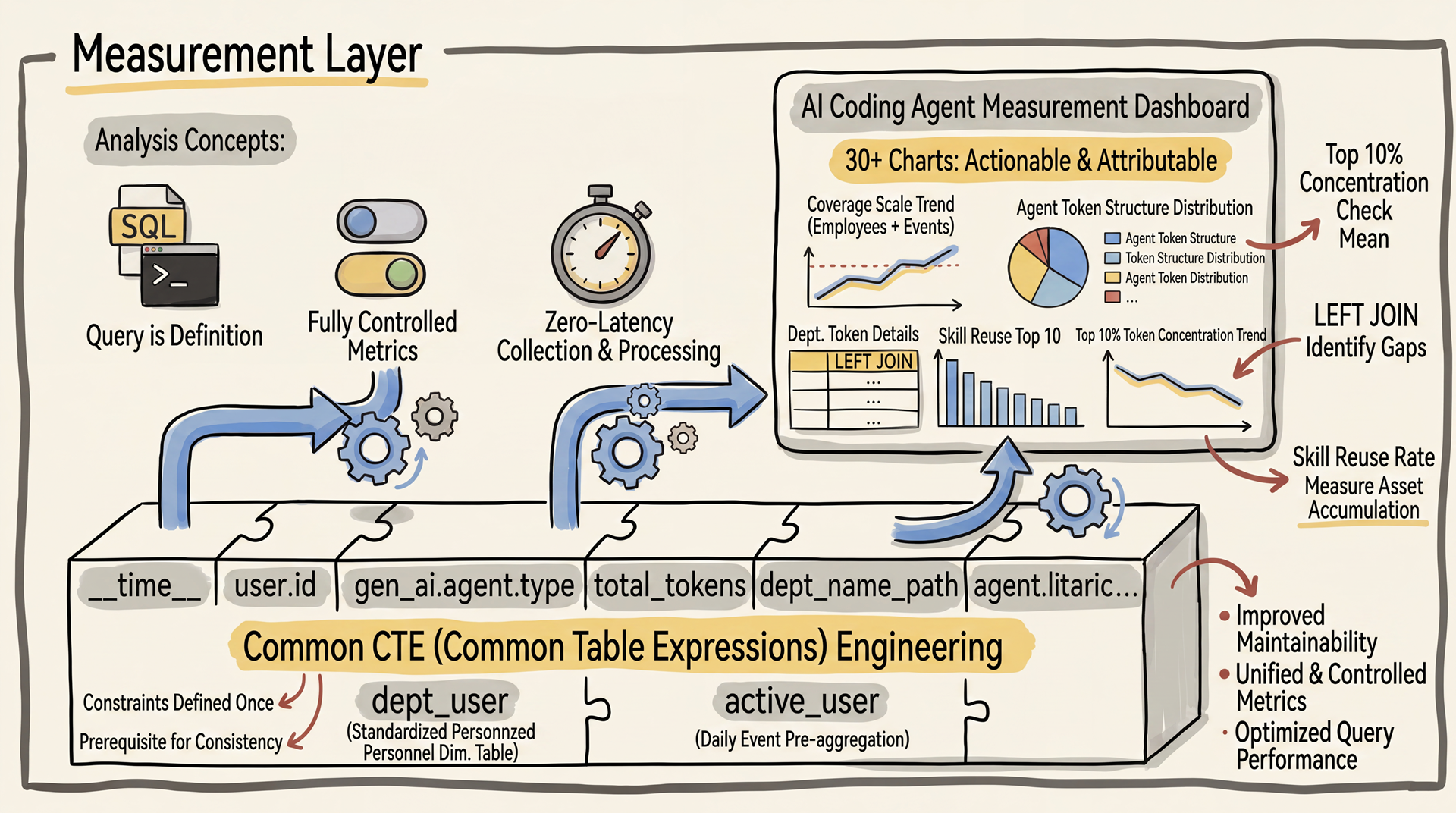
After having the data foundation, the next step is to choose an analysis carrier. We directly build the entire measure dashboard on the SLS dashboard using SQL. The core reason for choosing this path is flexibility. AI coding measure is a scenario where the metric highly varies by team and requirements undergo fast iteration. The analysis layer must give users sufficient freedom.
First, query is definition. Behind each chart on an SLS dashboard is an SQL statement. If requirements change, you can modify the SQL statement to make the changes take effect immediately. You do not need to wait for the product to be published or for configuration support.
Second, definitions are fully self-controlled. "What counts as an active user", "how to break down departments", and "whether the denominator for the coverage rate is registered employees or all employees" — these definition choices vary by organization and have no ground truth. SLS SQL allows each team to flexibly define them based on their own business characteristics. Your organization can break down by level-3 departments, while mine breaks down by project groups. Your definition of active is "having events in the past 7 days", while mine is "having events in the past 30 days and Tokens > 1000". These differences can be expressed by a single WHERE clause at the SQL layer.
Third, collection and analysis are on the same platform. After events are delivered to SLS, they can be queried immediately. There is no additional extract, transform, and load (ETL) link or T+1 delay. For example, if you just connect a new Agent, you can confirm whether data flows in normally on the dashboard within a few minutes after it is published. The verification closed loop is extremely short.
After flexibility is established, the next question is: How to maintain definition consistency across 30+ charts?
Flexibility solves the problem of "whether it can be modified". However, if each chart on a dashboard with 30+ charts has its own SQL statement, definition inconsistencies and maintenance costs will quickly spiral out of control. Therefore, the engineering core lies in the design of the analysis hierarchy: from metric definition, to pre-aggregation, to dimension progression, and then to specific charts, each layer serves the next layer.
All charts on the entire dashboard share the same group of CTE. This is not an SQL trick, but the engineering prerequisite for the entire report to achieve "definition consistency, maintainability, and controllable performance".
WITH dept_user AS (
SELECT
work_no,
show_name,
COALESCE(SPLIT_PART(dept_name, '-', 1), '') AS dept_name_1, -- Level-1 department, such as "Technology R&D Department"
COALESCE(SPLIT_PART(dept_name, '-', 2), '') AS dept_name_2, -- Level-2 department, such as "Engineering Platform Department"
COALESCE(SPLIT_PART(dept_name, '-', 3), '') AS dept_name_3 -- Team, such as "Data Service group"
FROM <dept-logstore>
GROUP BY work_no, show_name, dept_name
)
The core of this CTE is to break down the complete department path (such as Technology R&D Department-Engineering Platform Department-Data Service group) into a three-level hierarchy (level-1 department/level-2 department/team). The definition constraint of "statistics scope" is defined only once here. All downstream charts automatically inherit it through JOIN.
active_user AS (
 SELECT
 date_trunc('day', __time__) AS t,
 "user.id" AS user_id,
 coalesce(nullif("gen_ai.agent.type", 'null'), 'unknown') AS agent_type,
 coalesce(nullif("gen_ai.provider.name", 'null'), 'unknown') AS provider,
 coalesce(nullif("gen_ai.request.model", 'null'),
 nullif("gen_ai.response.model", 'null'), 'unknown') AS model,
 sum(coalesce("gen_ai.usage.input_tokens", 0)) AS input_tokens,
 sum(coalesce("gen_ai.usage.output_tokens", 0)) AS output_tokens,
 sum(coalesce("gen_ai.usage.total_tokens", 0)) AS total_tokens,
 count(1) AS events
 FROM <events-logstore>
 GROUP BY t, user_id, agent_type, provider, model
)
This CTE performs five-dimension pre-aggregation by day × user × Agent × supplier × model to produce the number of Tokens and events. The key benefit of pre-aggregation is: The vast majority of charts directly reuse active_user JOIN dept_user, and you do not need to repeatedly write aggregation logic for each chart.
Convention for JOIN between two tables:
FROM dept_user d
JOIN active_user a ON d.work_no = a.user_id
The design quality of the CTE layer determines three fundamentals of the entire dashboard: definition consistency (constraints are defined only once), maintainability (modifying one CTE automatically takes effect for all charts), and query performance (pre-aggregation reduces the scan volume of downstream SQL statements). For the 8 sections detailed later, the vast majority directly reuse CTE as the data source. A small number of charts that require finer granularity (such as Skill path fetch and repository dimension aggregation) revert to the original event table for separate queries. However, even so, the JOIN logic of the personnel dimension table still reuses dept_user to maintain definition consistency.
The 8 sections of the measure dashboard are not randomly stacked charts, but are designed progressively according to the analysis hierarchy:
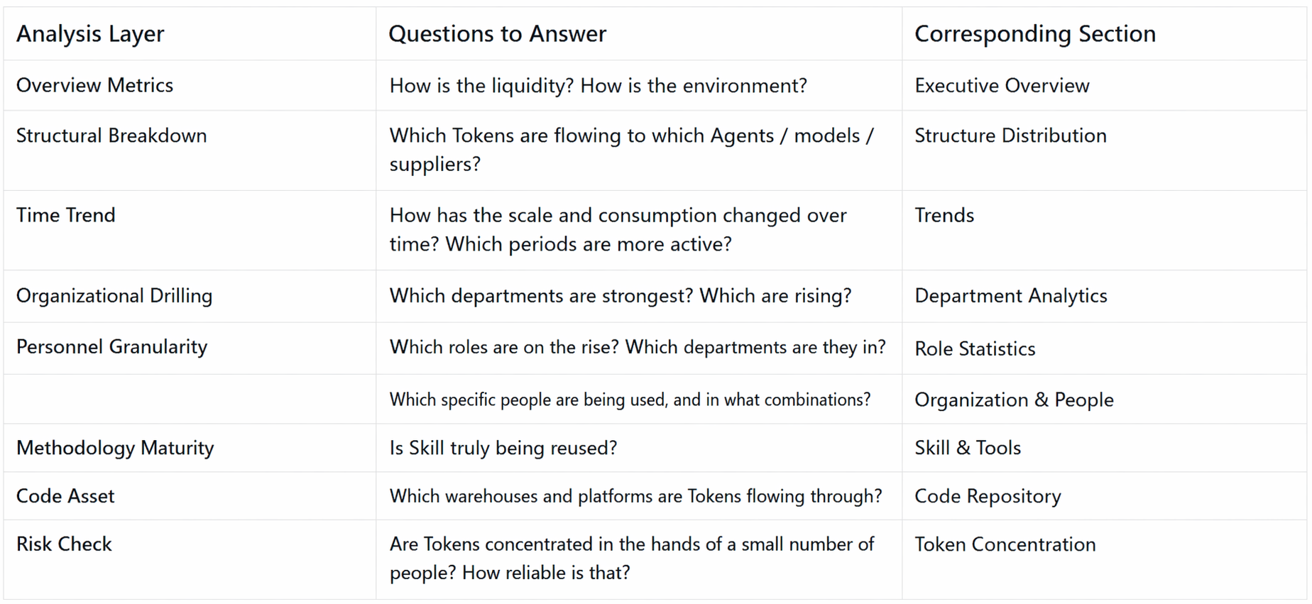
From "overall perception" to "structure breakdown" and then to "threat validation", each layer provides context for finer-granularity analysis.
The data in the following screenshots is all analog data, which is used to illustrate the report structure and analysis logic, and does not represent real business data.
A row of comparison cards at the top serves as the 'water level gauge' for the entire dashboard: active employees, total tokens, session count, Agent events, tokens per capita, and employees without reported usage. Each card includes a week-over-week (WoW) comparison against the same period last week. Together, these cards elevate the question of "how much is being used" from individual perception to the organizational level—revealing how many people are actively using it and whether overall usage this week is trending up or down compared to last week.
Cards showing abnormal week-over-week changes serve as drill-down entry points: if a metric drops, you can navigate to the corresponding section to identify the root cause. This shifts management decisions from intuition-driven to evidence-based.

To ensure WoW figures are reliable, the WoW calculation needs to work around a common pitfall: compare() is not compatible with cross-table CTE joins, and will throw an error directly. To address this, the calculation is instead implemented using manual windowing:
time_base AS (
  SELECT max(__time__) AS t_max FROM <event table>
),
cur_agg AS (
  SELECT "user.id" AS user_id, count(*) AS events
  FROM <event table>
  WHERE __time__ >= (SELECT t_max - 604800 FROM time_base)
  GROUP BY "user.id"
),
prev_agg AS (
  SELECT "user.id" AS user_id, count(*) AS events
  FROM <event table>
  WHERE __time__ >= (SELECT t_max - 1209600 FROM time_base)
    AND __time__ < (SELECT t_max - 604800 FROM time_base)
  GROUP BY "user.id"
)
-- JOIN dept_user separately and compute the WoW comparison after aggregation
SELECT
  cur.cnt AS "Current value",
  CASE WHEN prev.cnt > 0
       THEN round((1.0 × cur.cnt / prev.cnt - 1) × 100, 2)
  END AS "Compared to last week (%)"
FROM cur, prev
The SQL is longer, but it's the only reliably stable syntax under the "CTE + JOIN" architecture.
Three pie charts segment the token proportion by agent_type, model, and provider respectively, answering the resource configuration questions at the organization layer: which Agent is taking the lead, whether tokens are concentrated in one supplier or scattered among multiple suppliers, and what the main model of the team is. The answers directly determine whether the tools require convergence, how suppliers are centrally procured, and how costs are aggregated.
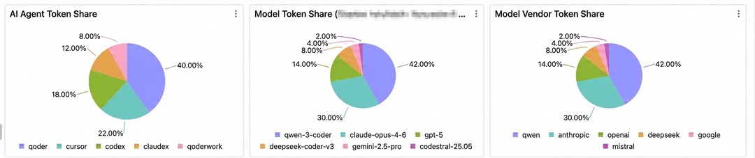
The data required for these decisions becomes very lightweight to obtain thanks to the CTE base: all three graphs run on dept_user JOIN active_user, and only the GROUP BY fields are different:
SELECT
  a.agent_type AS "AI Agent",
  sum(a.total_tokens) AS "Total tokens"
FROM dept_user d
JOIN active_user a ON d.work_no = a.user_id
GROUP BY a.agent_type
ORDER BY "Total tokens" DESC
Pre-aggregation allows each chart to focus solely on its own GROUP BY dimension, and switching model or provider versions is simply a matter of changing a single field.
Trend charts extend the "current status" to the "trend": the coverage size trend (a double line for the number of employees and the number of events), the Token consumption trend (three lines for input/output/total), the event and Token trends of each Agent (grouped by agent_type), and the distribution of Token usage time periods.
You can only make judgments from trends on whether the usage size of AI tools is steadily growing or falling back after a wave of promotion, and whether a specific Agent is becoming increasingly important or gradually overridden. The time period distribution provides a profile of the work rhythm. If Tokens are concentrated in the early morning, it indicates that the proportion of AI automation jobs is increasing. This is a completely different pattern from the usage driven by manual interaction during working hours, and the management actions are also different.
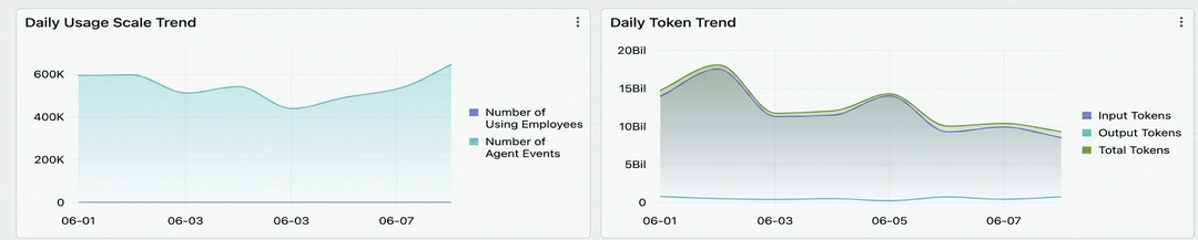

Most line charts can directly reuse the day granularity GROUP BY a.t of active_user. However, the time period distribution is an exception. The active_user has already been processed with date_trunc('day', __time__), and the hour dimension is discarded. To revert the hourly distribution, you must bypass the CTE and start a new hourly_user for independent aggregation:
hourly_user AS (
  SELECT
    date_format(__time__, '%H:00') AS h,
    "user.id" AS user_id,
    sum(coalesce("gen_ai.usage.total_tokens", 0)) AS total_tokens
  FROM < event table>
  GROUP BY h, user_id
)
SELECT a.h AS t, sum(a.total_tokens) AS "tokens"
FROM dept_user d
JOIN hourly_user a ON d.work_no = a.user_id
GROUP BY a.h
ORDER BY t
This is a typical backoff path when the downstream chart requires a finer granularity than the CTE.
Department statistics shift the perspective from individuals to teams. The department Token fact table (department, total number of people, number of users, coverage rate %, number of events, input/output/total Tokens, and Tokens per capita) is paired with the "list of employees who did not normally upload statistics data". Then, a Top 10 horizontal bar chart is overlaid, with sorting applied by total Tokens, coverage rate, and Tokens per capita, respectively.
The three dimensions point to three different actions: departments with a low size need promotion, departments with a low coverage rate need to be advanced from "individual early adoption" to "team standard", and departments with a low per capita usage may require optimization of tool configurations or improvement in usage methods.
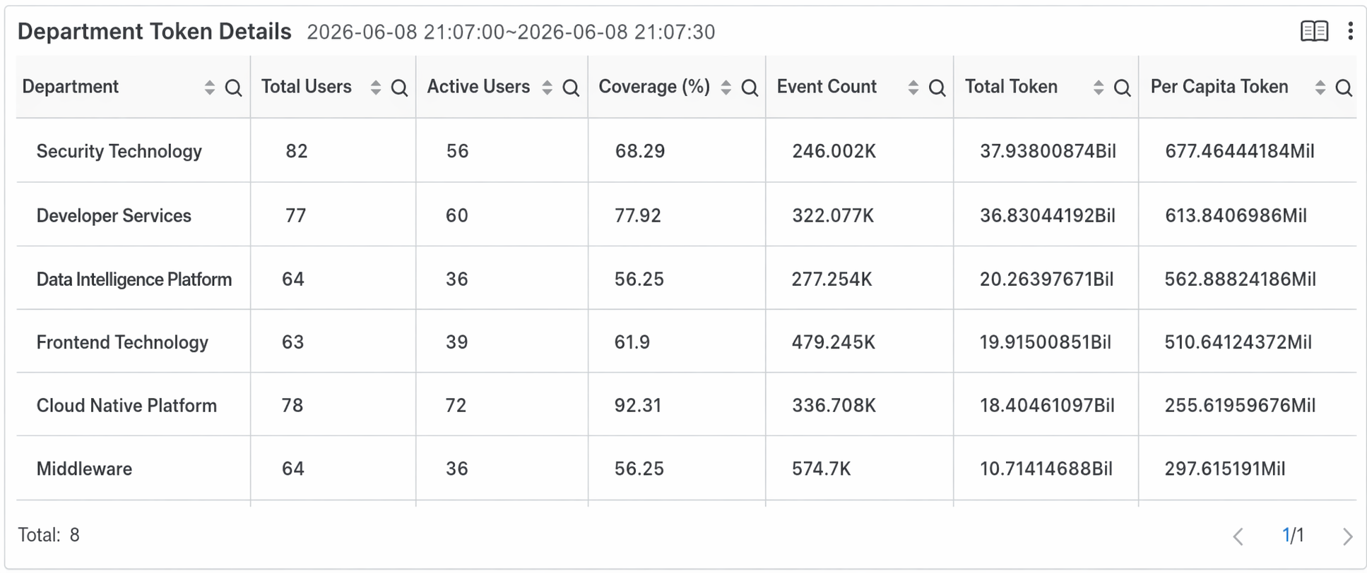
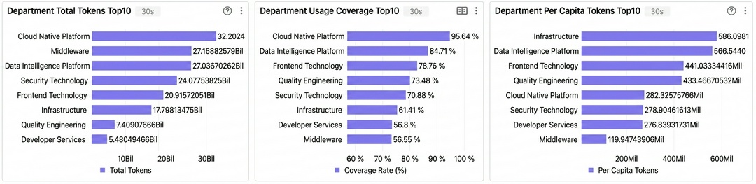
To make these rankings meaningful, departments with "0 users" cannot be filtered out, because they are exactly the targets of promotion. Therefore, the fact table uses LEFT JOIN instead of INNER JOIN:
SELECT
  d.dept_name_2 AS "Department",
  approx_distinct(d.work_no) AS "Total number of people",
  approx_distinct(a.user_id) AS "Number of users",
  round(100.0 × approx_distinct(a.user_id) / nullif(approx_distinct(d.work_no), 0), 2) AS "Coverage rate (%)",
  sum(a.total_tokens) AS "Total Tokens",
  round(1.0 × sum(a.total_tokens) / nullif(approx_distinct(a.user_id), 0), 2) AS "Tokens per capita"
FROM dept_user d
LEFT JOIN active_user a ON d.work_no = a.user_id
GROUP BY d.dept_name_2
ORDER BY "Total Tokens" DESC
LEFT JOIN allows departments with "0 users" to be retained in the table. These departments will not be silently filtered out by INNER JOIN. The "unreported" list is the same JOIN with the addition of WHERE a.user_id IS NULL. A single JOIN simultaneously supports two classes of outputs: "size ranking" and "blank search". The latter often drives organization action more effectively than the former.
This section penetrates from "department" to "individual": employee Token details (name/employee ID/team/Token/number of events/used AI Agents and models), AI agent details (Tokens and number of employees aggregated by agent_type), and model details (aggregated by model).
"Exactly who is using it, what combinations they use, and how deeply they use it" form the factual basis for team owners to conduct one-on-one coaching and tool recommendations. The AI Agent/model details aggregate individual behaviors into tool profiles. This feeds back into tool selection and the accumulation of best practices.
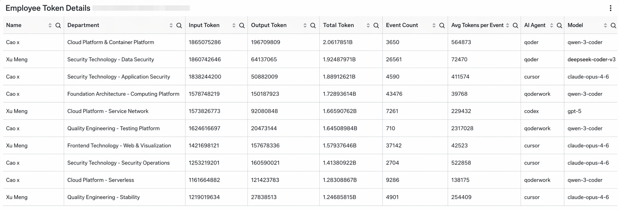
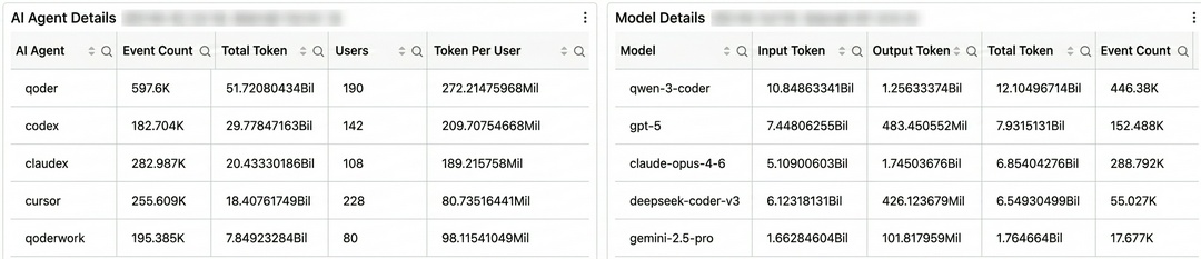
Because you want to view "which agents/models a person has used", you need to aggregate multiple values into readable fields. The common syntax is to simply use array_agg(DISTINCT …). However, to ensure that the weekly report comparison does not generate noise, you must add another layer of array_sort to guarantee the stability of the outputs. Without this step, the exported CSV file will generate a large amount of noise between two differences because of the random jitter in the order of array elements.
SELECT
  d.show_name AS "Name",
  d.work_no AS "Employee ID",
  d.dept_name_2 AS "Team",
  sum(a.total_tokens) AS "Total tokens",
  sum(a.events) AS "Number of events",
  round(1.0 × sum(a.total_tokens) / nullif(sum(a.events), 0), 2) AS "Average tokens per event",
  array_join(array_sort(array_agg(DISTINCT a.agent_type)), ', ') AS "AI Agent",
  array_join(array_sort(array_agg(DISTINCT a.model)), ', ') AS "Model"
FROM dept_user d
JOIN active_user a ON d.work_no = a.user_id
GROUP BY d.show_name, d.work_no, d.dept_name_2
ORDER BY "Total tokens" DESCThe three Top 10 vertical bar charts for the number of Skill calls, the number of Skill users, and the number of Tool calls constitute the most distinctive segment in the entire dashboard. The number of calls indicates the intensity with which a single Skill is used, and the number of users indicates its spread breadth within the team. A Skill with both high numbers is a methodology that is truly accumulated as an organization asset. A Skill with a high number of calls but a low number of users remains in the individual exploration stage.
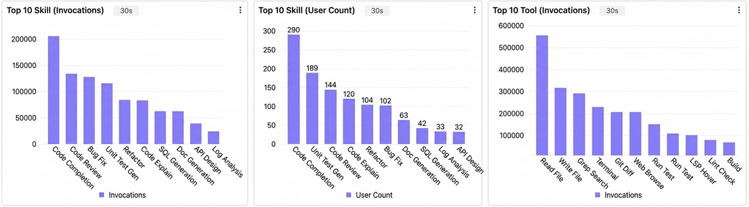
However, to retrieve these rankings, you must first extract the Skill name from the file path. This itself is the most core SQL logic in this section. SKILL.md has many variations under the history folder structure (skills/<name>/SKILL.md, skills/<name>/v1.2/SKILL.md, and .qoderwork/<name>.skill.md). The fetch rules are as follows:
SELECT skill_name AS "Skill", count(1) AS "Number of calls"
FROM (
  SELECT
    CASE
      -- If the candidate is a version number, fetch another segment of the folder name upwards
      WHEN regexp_like(regexp_extract(path, '/([^/]+)/[^/]+$', 1), '^v?[0-9]+\.[0-9]+')
      THEN regexp_extract(path, '/([^/]+)/v?[0-9][^/]*/[^/]+$', 1)
      -- The candidate is the container folder name → fetch from the file name, and remove the suffix
      WHEN lower(regexp_extract(path, '/([^/]+)/[^/]+$', 1))
           IN ('skills','skill','.claude','agents','resources','.qoderwork','docs')
      THEN regexp_replace(regexp_extract(path, '/([^/]+)$', 1), '(?i)(\.skill)?\.md$', '')
      -- Default: take the folder name of the second to last segment
      ELSE regexp_extract(path, '/([^/]+)/[^/]+$', 1)
    END AS skill_name
  FROM <event table> t
  JOIN dept_user d ON t."user.id" = d.work_no
  WHERE regexp_like(t."gen_ai.tool.call.arguments.file_path",
'(?i)(/SKILL\.md|/[^/]+\.skill\.md)$')
)
WHERE skill_name IS NOT NULL AND skill_name <> '' AND upper(skill_name) <> 'SKILL'
GROUP BY skill_name
ORDER BY "number of calls" DESC LIMIT 1
Bypass the entire active_user, and directly JOIN the original event table, because gen_ai.tool.call.arguments.file_path is not in the CTE.
If Skills answer "whether the methodology is reused", the repository answers "which code assets the AI-assisted coding investment actually flows into". The Repo Token Top10 horizontal bar chart and the Git Domain Token proportion pie chart provide two dimensions: whether tokens flow centrally into core business repositories or are scattered across experimental projects, and whether they are mainly consumed in internal GitLab (controlled assets) or external GitHub (code outside the border).
These two distributions directly serve the judgment of "whether the AI investment is aligned with the organizational strategy".
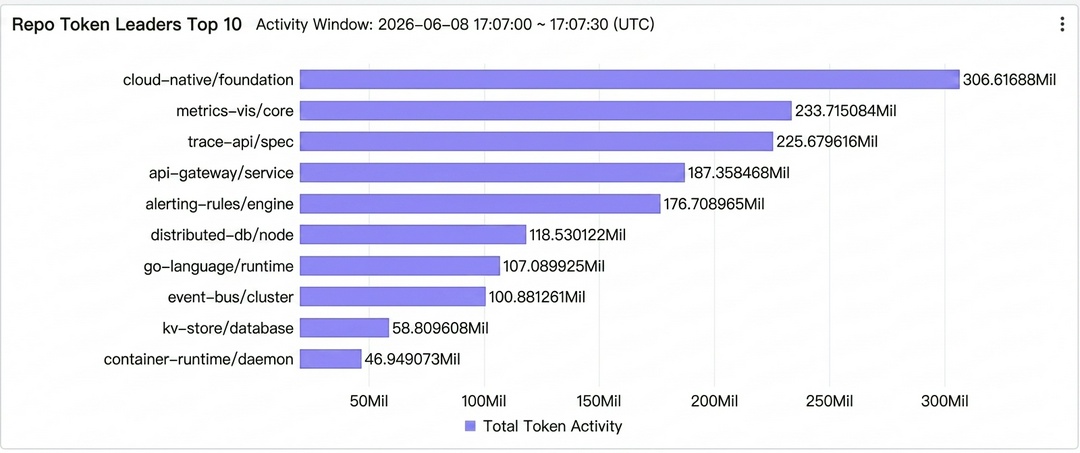
To support this perspective, an architectural trade-off must be resolved: git.repo and git.domain cannot enter the active_user CTE. If you add the repository to GROUP BY, the number of CTE rows expands from "person × day" to "person × day × repository", which instead slows down all downstream charts. Therefore, we revert to the original event table here to aggregate separately:
SELECT
  coalesce(nullif(t."git.repo", ''), 'unknown') AS "repository",
  sum(coalesce(t."gen_ai.usage.total_tokens", 0)) AS "Total Tokens"
FROM <event table> t
JOIN dept_user d ON t."user.id" = d.work_no
WHERE t."git.repo" IS NOT NULL AND t."git.repo" != ''
GROUP BY "repository"
ORDER BY "Total Tokens" DESC LIMIT 10
This is an example of "which dimensions should enter the CTE and which should be left out": a general pre-aggregation is not necessarily better just because it is wider.
Concentration is the most direct validation for all previous "total amount" metrics. When the "Tokens per capita" in Section 1 looks impressive, you must ask whether it is a benefit for all employees or a mean supported by a few top individuals. If the top 10% of individuals account for more than 70% of the tokens, the organization remains at the stage of "individual productivity of a few people" even if the total amount is large.
Numeric cards (top 10% or top 20% token proportion), audience layered vertical bar charts (three buckets: top 10%, 10% to 20%, and the bottom 80%), and daily concentration trend lines combine to answer "whether the concentration is improving or deteriorating." A continuous decrease in concentration means that AI coding is diverging from an individual capability to a common capability of the organization.
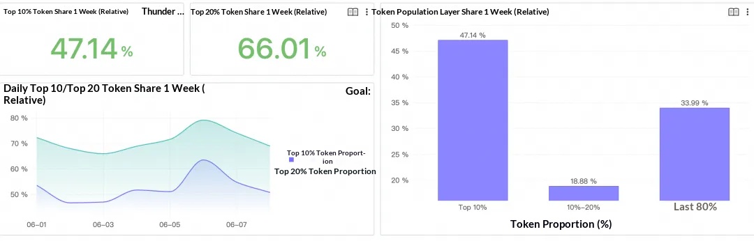
The key to making this judgment is to use a window function for ranking and then create buckets by percentile:
user_token AS (
  SELECT a.user_id, sum(a.total_tokens) AS total_tokens
  FROM dept_user d
  JOIN active_user a ON d.work_no = a.user_id
  GROUP BY a.user_id
  HAVING total_tokens > 0
),
ranked AS (
  SELECT user_id, total_tokens,
    row_number() OVER (ORDER BY total_tokens DESC) AS rn,
    count(*) OVER () AS user_count,
    sum(total_tokens) OVER () AS all_tokens
  FROM user_token
)
SELECT
  round(100.0 × sum(CASE WHEN rn <= cast(ceil(user_count × 0.1) AS bigint)
                         THEN total_tokens ELSE 0 END)
              / max(all_tokens), 2) AS "Top 10% Token Proportion"
FROM ranked
The daily trend version only has one additional PARTITION BY t, which changes "global ranking" to "ranking per day." cast(ceil(user_count × 0.1) AS bigint) ensures that the top 10% border can be correctly retrieved even if the total number of people is not divisible.
The answer provided in this topic is a three-layer progressive path:
Layer 1: unified semantics collection. The LoongSuite GenAI semantics specification solves the problem of "what standard to use for records," and LoongSuite-Pilot solves the problem of "how to collect from heterogeneous agents." Regardless of whether you use Claude Code, Copilot, or Cursor, events are written to SLS based on the same field structure, making the events comparable across tools and traceable across time.
Layer 2: Flexible analysis. The SLS dashboard uses SQL as the unique definition language. The calculation methods are completely self-controlled and can be queried in seconds. Public CTEs serve as the engineering foundation. This guarantees the calculation method consistency and maintainability of 30+ charts. From overview to structure, from trend to personnel, and from skill reuse to code repository and token concentration degree, the eight sections progress according to the analysis layers. Each layer provides context for judgments of finer granularity.
Layer 3: Actionable organization. The personnel dimension table exposes the empty areas of "registered but not reporting" through a LEFT JOIN. The concentration degree dashboard validates whether the per capita metrics are supported by top individuals. These are not just good-looking numbers. They are signals that can be directly converted into actions.
AI is an amplifier. The value of the measure layer is to let the organization clearly see what it is amplifying, and then decide where to go next.
[1] DORA: ROI of AI-Assisted Software Development — Google Cloud
https://cloud.google.com/resources/content/dora-roi-of-ai-assisted-software-development
[2] ROI of AI-Assisted Software Development report — DORA.dev
https://dora.dev/ai/roi/report/
[3] LoongSuite GenAI semantics specification — GitHub
https://github.com/alibaba/loongsuite-semantic-conventions-genai/
[4] OpenTelemetry GenAI semantic conventions — OpenTelemetry
AgentTeams and Claude Tag Both Enter Group ChatMode: Is it a New Paradigm or a New Narrative?
One Single Source of Truth to End Skill Management Chaos: Best Practices for Skill Governance

780 posts | 60 followers
FollowAlibaba Cloud Native Community - July 23, 2026
Alibaba F(x) Team - September 30, 2021
Alibaba Clouder - March 10, 2021
Alibaba Cloud Community - July 17, 2026
Bryan, Zhang - June 17, 2026
Alibaba Cloud Native Community - January 4, 2026
780 posts | 60 followers
Follow Token Plan
Build more, spend less. One plan, every modality.
Learn More QwenWork
QwenWork is dedicated to helping employees strengthen their professional competitiveness in the AI era and to enabling enterprises to improve organizational effectiveness.
Learn More
Alibaba Cloud Model Studio
A one-stop generative AI platform to build intelligent applications that understand your business, based on Qwen model series such as Qwen-Max and other popular models
Learn More DevOps Solution
Accelerate software development and delivery by integrating DevOps with the cloud
Learn MoreMore Posts by Alibaba Cloud Native Community

