This article is organized from the sharing of the AI feature engineering session of FFA 2023 by Weibo Zhao. The content is divided into the following four parts:
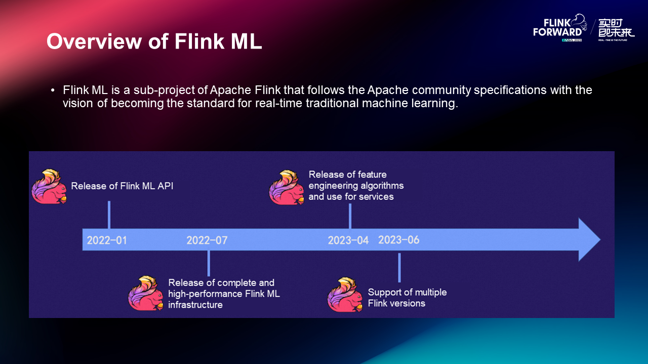
Flink ML is a sub-project of Apache Flink that follows the Apache community specifications with the vision of becoming the standard for real-time traditional machine learning.
The Flink ML API was released in January 2022, followed by the launch of a complete, high-performance Flink ML infrastructure in July 2022. In April 2023, feature engineering algorithms were introduced, and support for multiple Flink versions was added in June 2023.
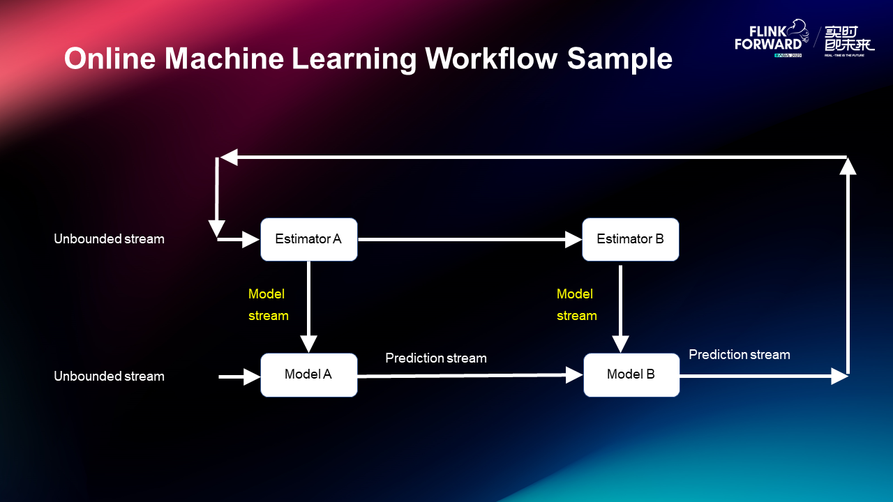
There are two models A and B which are trained by online learning and used for online inference. In the inference process, this model is in the form of a stream. That is the model stream which continuously flows the model into the chain so that the model has better real-time performance. After the inference is completed, the inference sample will be recommended to some front customers. Then the customers will give feedback on the results. Some samples will be spliced, and finally returned to the training data stream to form a closed loop. That is the workflow sample.
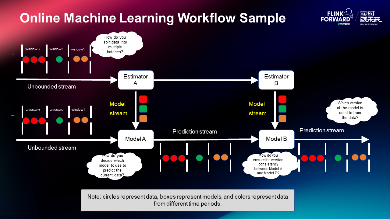
Next, the design of online learning is introduced with a workflow sample. The training data is cut into different windows after splitting. Each window needs to update the model when it passes through the Estimator, and then the model will flow to the inference chain below. As the data continues to flow, the model will flow to the inference chain one by one. This is the model stream whose idea is to support inference by turning the model into a queue to achieve better real-time performance.
Problems:
There are four design requirements for four questions:
To fulfill these requirements, our design plan includes:
1. Add the HasWindows interface.
Users are allowed to declare different policies for partitioning data.
2. Add the model version and timestamp for ModelData. The value of the model version starts from 0 and increases by 1 each time. The timestamp of the model data is the maximum timestamp of the data from which the model is trained.
3. Add HasMaxAllowedModelDelayMs interface.
When users are allowed to specify the prediction data D, the time when the model data M is earlier than D is less than or equal to the set threshold.
4. Add HasModelVersionCol interface. During inference, users are allowed to output the model version used when predicting each piece of data.
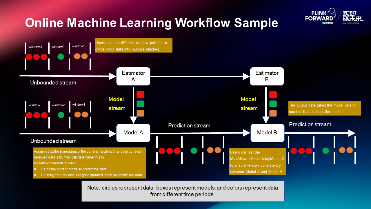
Let's come back and look at the problem after we have the plan:
Then, the first four problems can be solved.
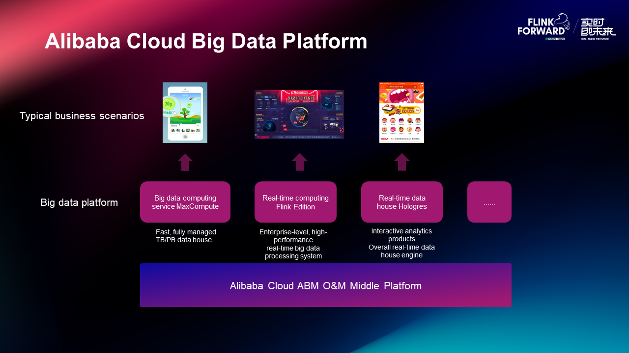
Alibaba Cloud ABM O&M Middle Platform collects logs from all Alibaba platforms, clusters the error logs, and sends the error logs to the corresponding department for subsequent processing.
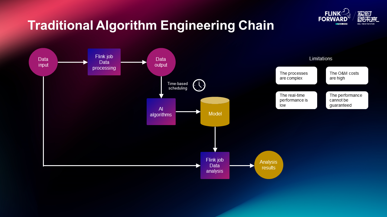
Traditional algorithm engineering chains first input data and use Flink job for data processing. The data will be dropped to the disk. Then, the clustering algorithm will be pulled up through timing scheduling. The model is written to pull up the Flink job for data prediction through loading. However, the whole chain has limitations of complex processes, high O&M cost, low real-time performance, and the performance cannot be guaranteed.
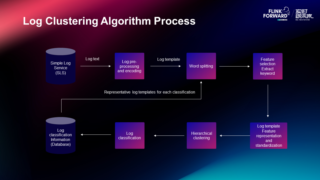
The log clustering algorithm process splits words after pre-processing and encoding the system logs. It extracts keywords through feature selection, performs feature representation and standardization of the logs, and then performs hierarchical clustering and log classifications. It finally writes them to the database to guide word splitting.
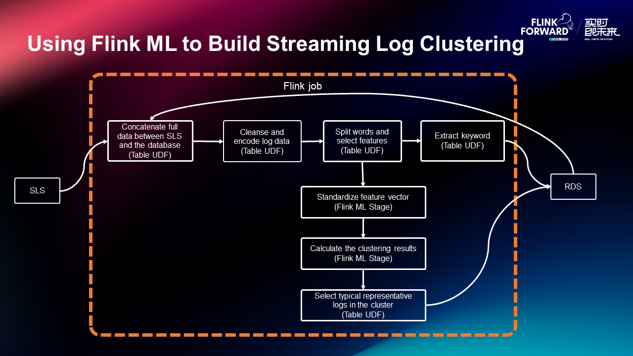
For this process, we can use Flink ML to build streaming log clustering to string this process. A Flink job is used to concatenate full data between SLS and the database. Next, log data is cleansed and encoded. Then, word splitting and standardization are performed to calculate the clustering results. Finally, typical representative logs in the cluster are selected.
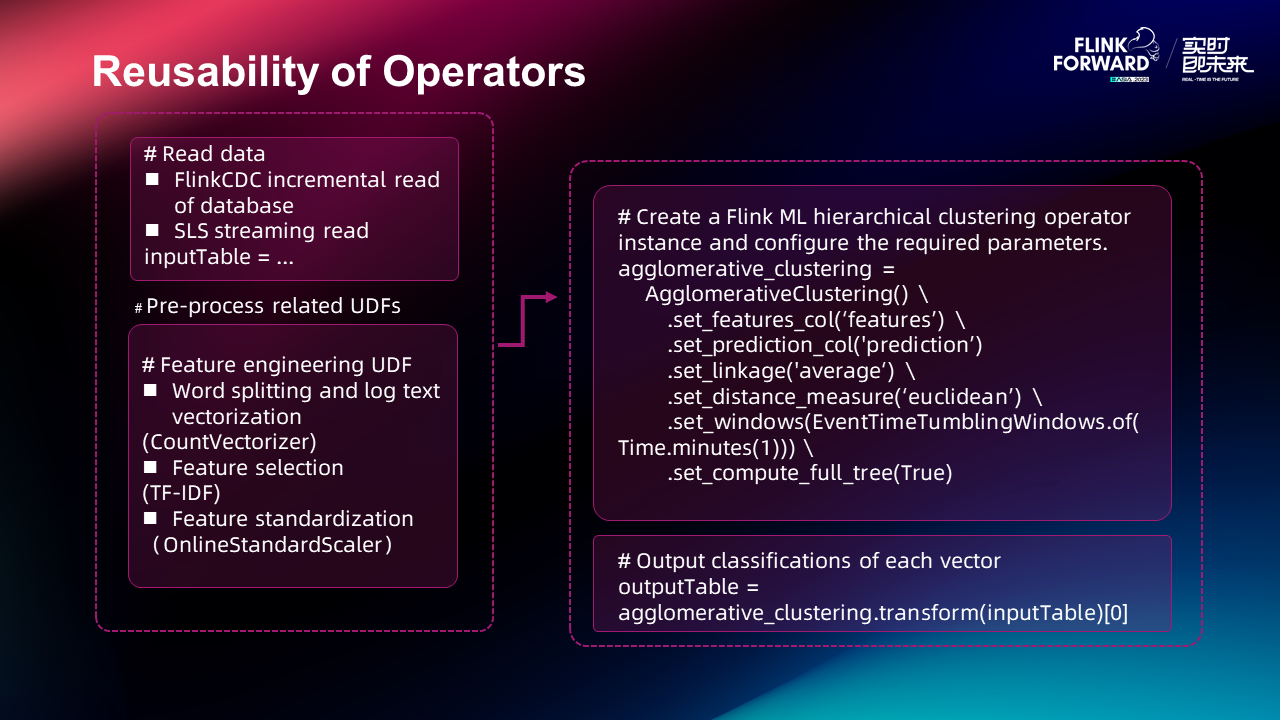
You can extract the operators in this case, such as SLS streaming reading, word splitting, log vectorization, feature selection, and feature standardization. These operators are not unique to the business but are required by many online learning businesses. If you extract them into an independent component, customers can reuse these operators when they need to do online learning processes.
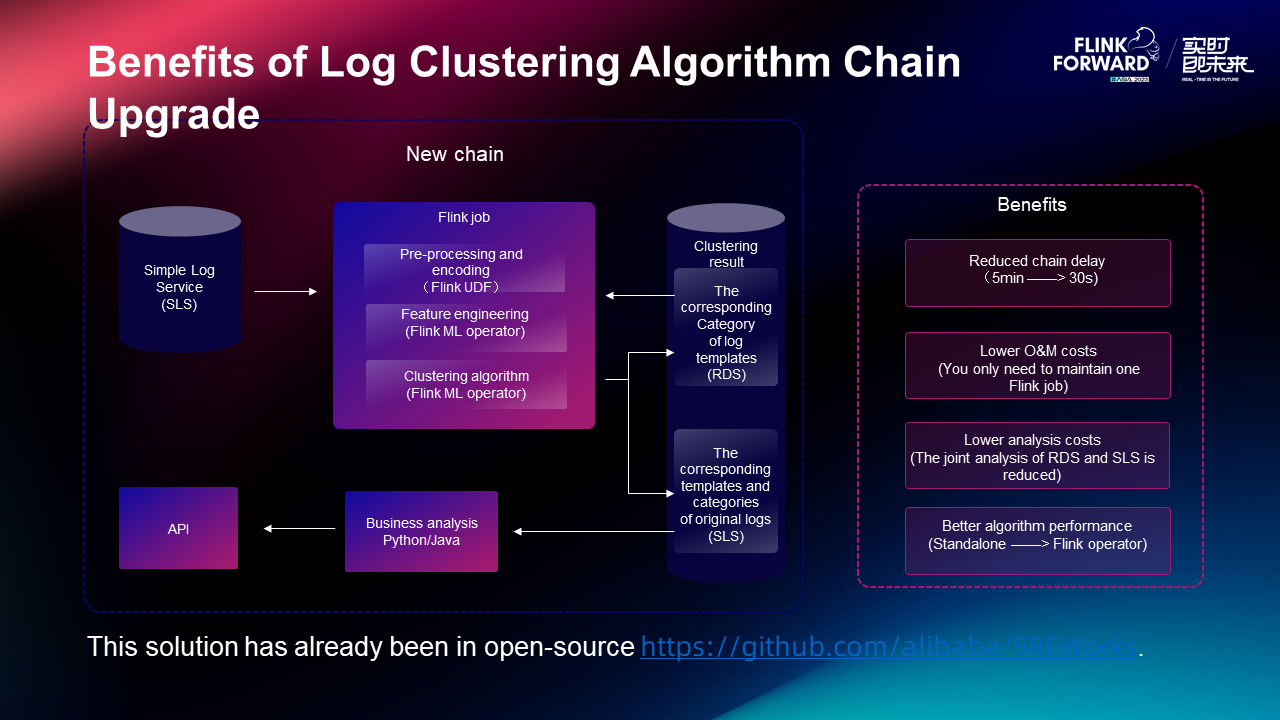
Benefits of log clustering algorithm chain upgrade:
• In terms of chain delay, the original delay of 5 minutes is reduced to 30 seconds.
• Operating costs are reduced, and now only one Flink job needs to be maintained.
• The analysis costs are reduced.
• The algorithm performance is improved.
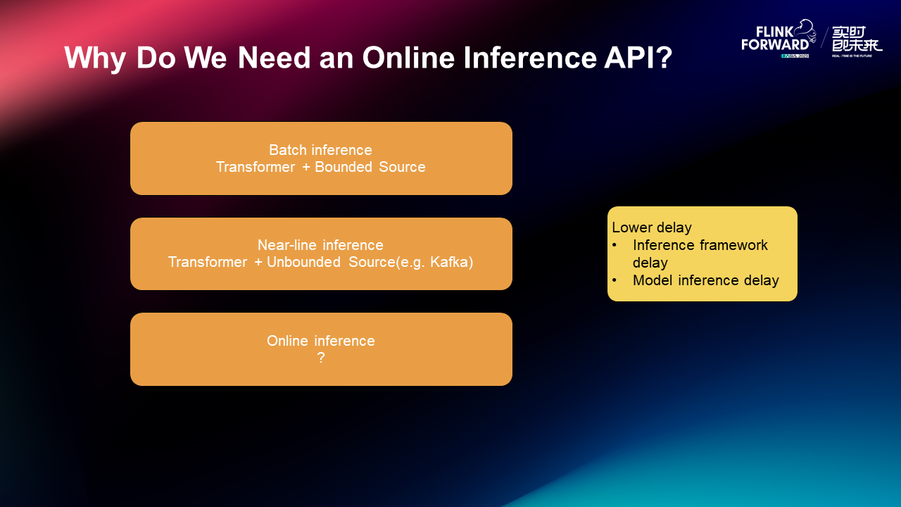
The inference is mainly divided into the following:
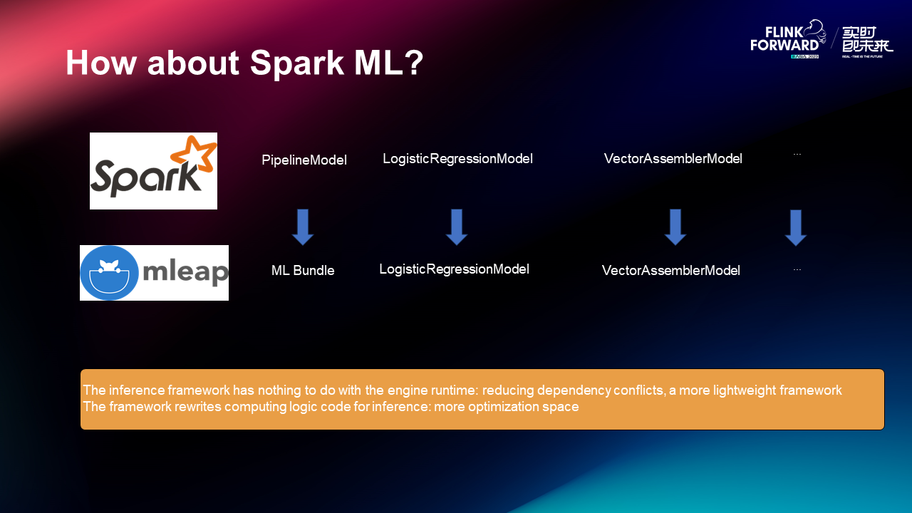
Before doing this, we surveyed the Spark ML inference. Later, it is found that Spark ML itself does not have an inference module. It has an Mleap which makes Spark inference into an inference framework. This inference framework has nothing to do with the engine runtime and reduces dependency conflicts. It is a lighter framework. In addition, this new framework can rewrite computing logic code for inference and has more optimization space.
The design requirements draw on Mleap's approach:
1. Data representation (independent of Flink Runtime)
• A single piece of data representation: Row
• Batch data representation: DataFrame
• Data type representation: providing support for Vector and Matrix
2. Inference logic representation
3. Model loading
• It supports loading from files of Model/Transformer# save
• It supports dynamic loading of model data without the need to restart
4. Utils
• It supports checking whether Transformer/PipelineModel supports the online inference
• It concatenates multiple inference logic into a single inference logic
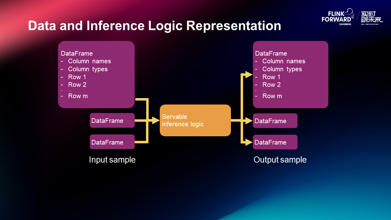
Under this design requirement, on the left is the inference data structure DataFrame which contains column names, column types, and rows. After entering the inference logic, the output is of the same data structure, so that the entire inference structure can be strung together without data structure conversion.
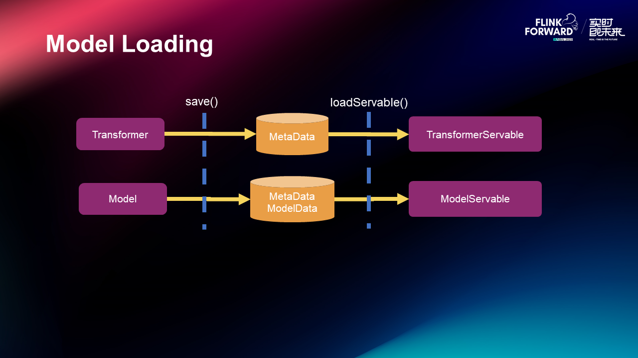
On the model loading side, the model is written to disk through the save function. The save() on the left is what Flink ML does, and the loadServable() on the right is what the inference framework does. Through these two functions, the model is saved, loaded, and inferred.
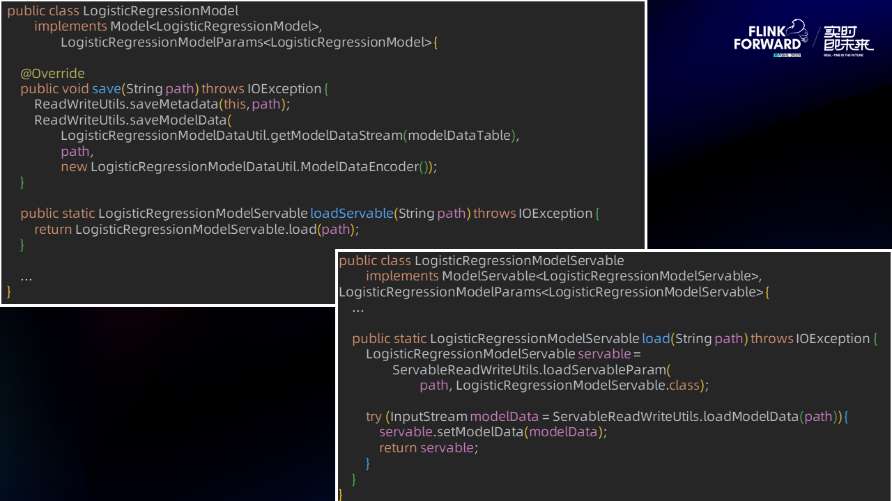
Next, let's take logic regression as an example to see the implementation of the code. The save function is used to write the model to the specified directory. The following load is what the inference framework does, and the file of the load model is used for inference.
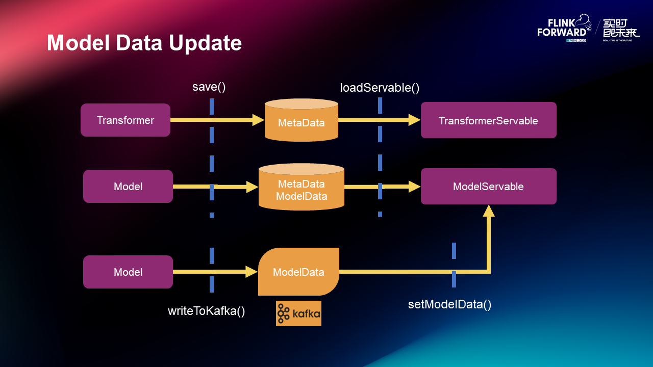
The data update of the model is to write a model into Kafka, and Kafka is set into the Servable of the model. When the model is written into Kafka, the model will naturally flow into the Servable and finally the dynamic update of the model is realized.
The codes are as follows
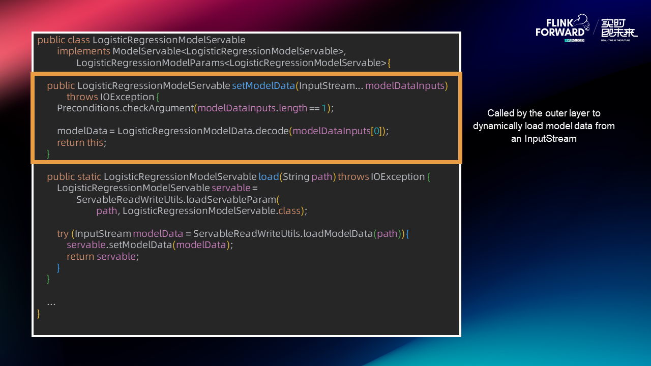
The input of setModelData is InputStream which can be read from Kafka. When the data in Kafka is updated, it can be updated to the model.
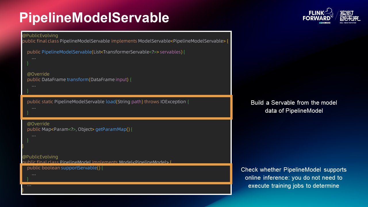
In addition, we also support PipelineModel inference. You can build a Servable from the model data of PipelineModel to check whether PipelineModel supports online inference. You can determine whether PipelineModel supports online inference without the need to execute training jobs.
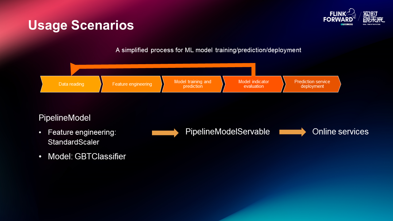
Finally, let's look at the usage scenarios. This is a simplified process for ML model training, prediction, and deployment. The initial step involves data ingestion, feature engineering, followed by evaluation and deployment. In this instance, the PipelineModel is used to encapsulate the two models of standardization and GBT classification into a Pipeline, enabling the execution of online inference services.
The codes are as follows
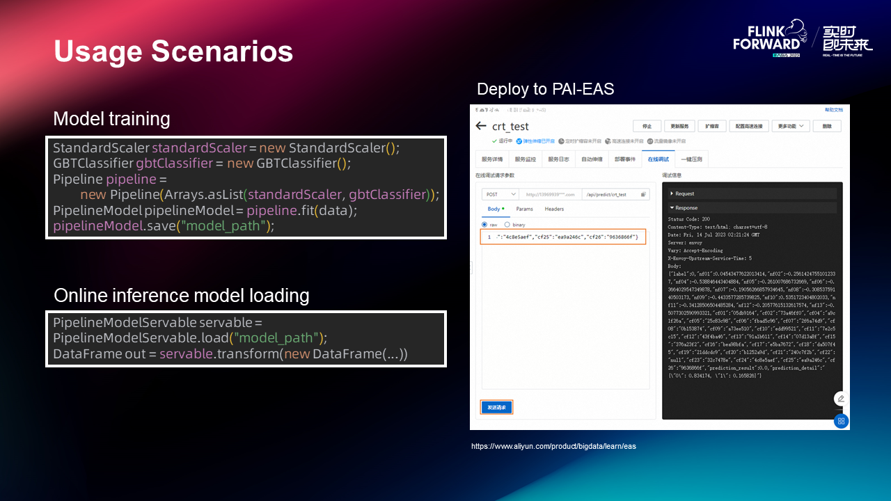
The standardization and GBT models are written through Pipeline, and the Pipeline inference is finally implemented in the inference module. The inference supports writing and dynamic loading.
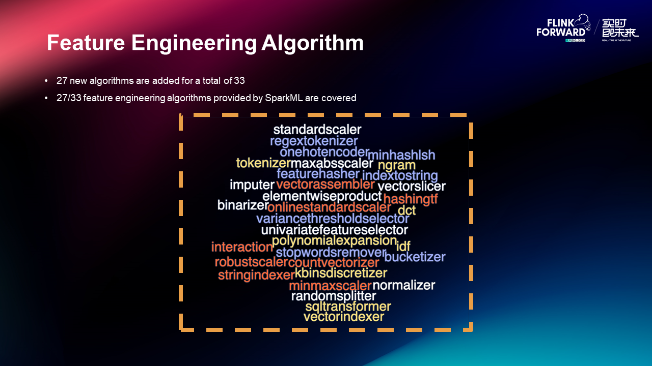
27 new algorithms have been added, bringing the total to 33, which now encompasses common algorithms.
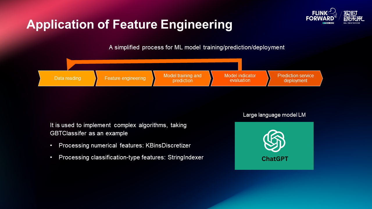
The first application scenario involves recommendation and advertising evaluation, both of which require feature processing. The second application scenario is to implement complex algorithms. For example, GBT is used to process numerical features and process classification-type features. Additionally, Flink ML has incorporated some designs for the large language model.
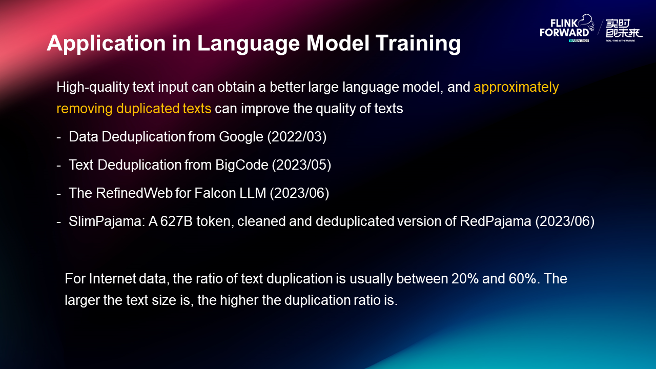
Next, let's use the large language model as an example to examine the business of feature engineering. A high-quality text input can result in a better large language model, and the approximate removal of duplicate texts can enhance text quality. In Internet data, the text duplication ratio typically falls between 20% and 60%, with larger text sizes associated with higher duplication ratios.
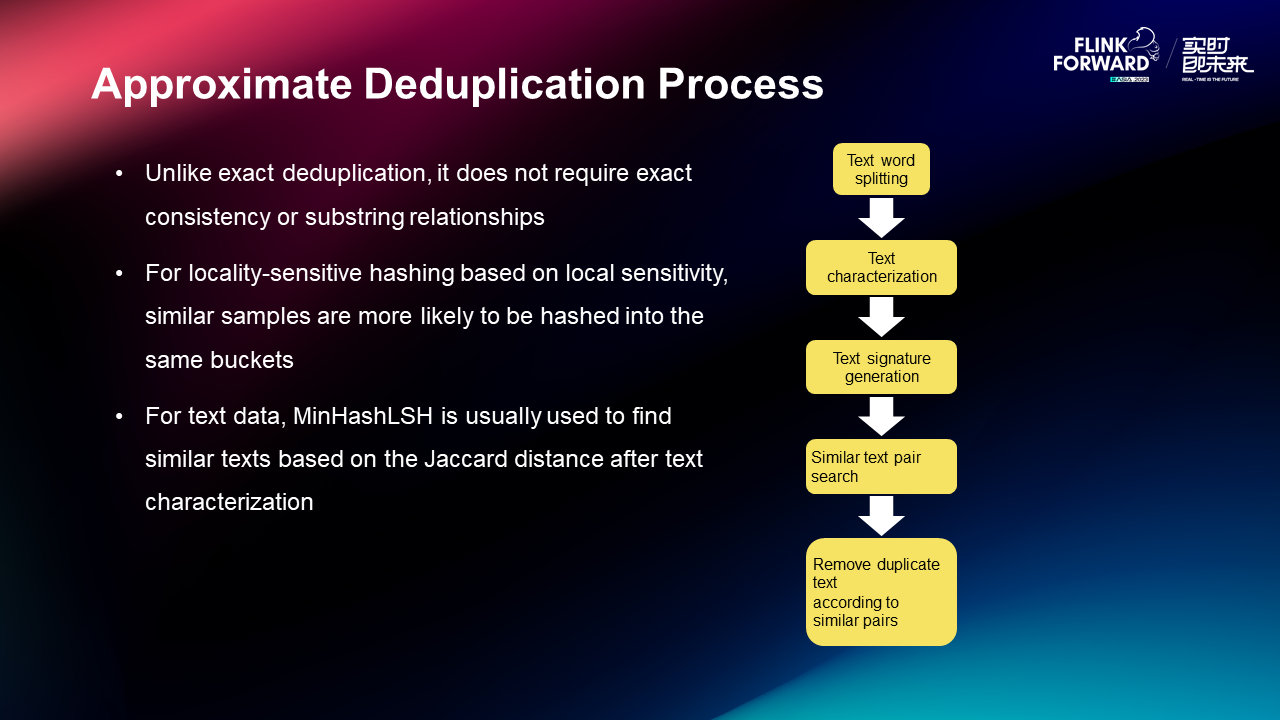
To solve this problem, we have designed an approximate deduplication process:
• Unlike exact deduplication, it does not require exact consistency or substring relationships.
• For locality-sensitive hashing based on local sensitivity, similar samples are more likely to be hashed into the same buckets.
• For text data, MinHashLSH is usually used to find similar texts based on the Jaccard distance after text characterization.
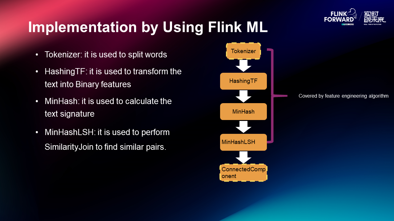
You can use these components to complete the text deduplication process:
• Tokenizer: it is used to split words
• HashingTF: it is used to transform the text into Binary features.
• MinHash: it is used to calculate the text signature.
• MinHashLSH: it is used to perform SimilarityJoin to find similar pairs.
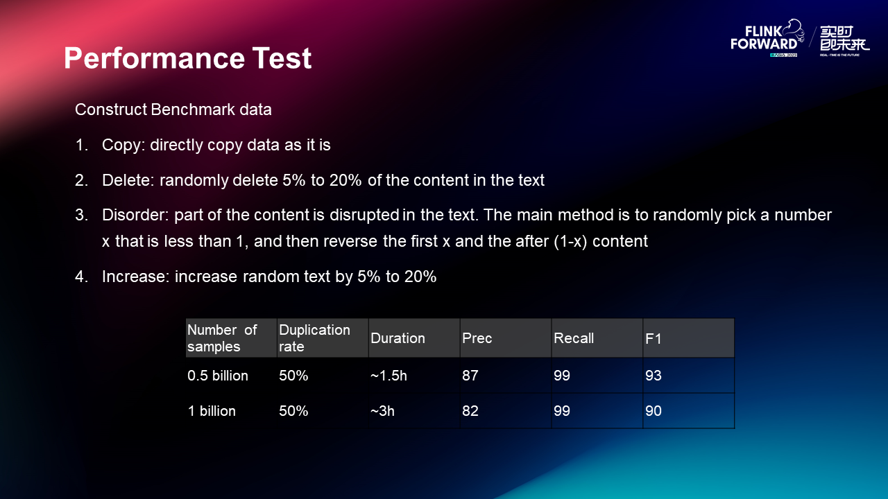
Finally, the performance test involved a manually constructed benchmark dataset obtained directly through copy and delete operations. For a dataset containing 500 million records with a 50% duplication rate, the deduplication process took approximately 1.5 hours.
Using Apache Paimon + StarRocks High-speed Batch and Streaming Lakehouse Analysis

206 posts | 56 followers
Follow5141082168496076 - February 20, 2020
Data Geek - May 9, 2023
Apache Flink Community China - September 27, 2020
Apache Flink Community China - December 25, 2019
Alibaba Cloud Community - March 9, 2023
Apache Flink Community - March 20, 2025

206 posts | 56 followers
Follow Realtime Compute for Apache Flink
Realtime Compute for Apache Flink offers a highly integrated platform for real-time data processing, which optimizes the computing of Apache Flink.
Learn More Big Data Consulting for Data Technology Solution
Alibaba Cloud provides big data consulting services to help enterprises leverage advanced data technology.
Learn More Big Data Consulting Services for Retail Solution
Alibaba Cloud experts provide retailers with a lightweight and customized big data consulting service to help you assess your big data maturity and plan your big data journey.
Learn More ApsaraDB for HBase
ApsaraDB for HBase is a NoSQL database engine that is highly optimized and 100% compatible with the community edition of HBase.
Learn MoreMore Posts by Apache Flink Community