In this article, the Alibaba Cloud Open-Source Big Data OLAP Team and the StarRocks Data Lake Analysis Team jointly introduce the principles of the StarRocks blazing-fast data lake analytics.
StarRocks is a powerful data analytics system whose main purpose is to provide blazing-fast, unified, and easy-to-use data analytics and help you quickly gain insight into the value of data at lower usage costs. With a streamlined architecture, an efficient vectorized engine, and a newly designed cost-based optimizer (CBO), the analytics performance of StarRocks, especially multi-table JOIN queries, is far superior to similar products.
The Alibaba Cloud Open-Source Big Data OLAP Team works with the community to meet the needs of more users for blazing-fast data analysis, apply the powerful analytics performance of StarRocks to a wider range of data sets, and enhance the capability of StarRocks for data lake analytics. It enables the data lake to analyze the data stored locally in StarRocks and the data stored in open-source data lakes or data warehouses, such as Apache Hive, Apache Iceberg, and Apache Hudi, with the same outstanding performance.
This article focuses on the technology, performance, and future planning of StarRocks' blazing-fast data lake analytics.
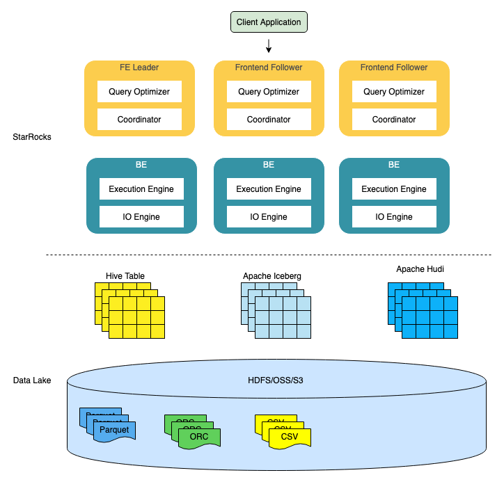
In the scenarios of data lake analytics, StarRocks is mainly responsible for data computing and analytics, while a data lake is mainly responsible for data storage, organization, and maintenance. The figure above depicts the completed technology stack composed of StarRocks and a data lake.
The architecture of StarRocks is very simple. The core of the entire system is only frontend (FE) and backend (BE) processes. The system does not rely on any external components, which facilitates deployment and maintenance. FE is mainly responsible for parsing query statements (SQL), optimizing queries, and scheduling queries, while BE is mainly responsible for reading data from the data lake and completing operations, such as filtering and aggregating.
A data lake is a collection of technical concepts. A common data lake usually contains three modules: table format, file format, and storage. The table format is the UI of a data lake. Its main feature is to organize structured, semi-structured, and unstructured data so those data can be stored in distributed file systems (such as HDFS) or Object Storage Service (such as OSS and AWS S3/Amazon Simple Storage Service), and the relevant semantics of the table structure can be exposed. The table format includes two major genres. One is to organize metadata into a series of files and store them together with actual data in a distributed file system or Object Storage Service. For example, Apache Iceberg, Apache Hudi, and Delta Lake all belong to this genre. Another is to use a customized metadata service to separately store metadata, such as StarRocks local tables, Snowflake, and Apache Hive.
The main function of file format is to provide data units with an expression that is convenient for efficient retrieval and compression. Currently, common open-source file formats include column-based Apache Parquet and Apache ORC, row-based Apache Avro, etc.
Storage is a module for storing data in a data lake. Currently, the most commonly used storage in a data lake is distributed file systems (such as HDFS) and Object Storage Services (such as OSS and AWS S3).
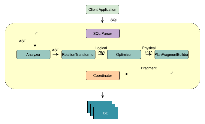
The main feature of FE is to convert SQL statements into fragments that BE can recognize. If a BE cluster is regarded as a distributed thread pool, fragments are tasks in the thread pool. From SQL texts to distributed physical execution plans, FE needs to go through the following steps:
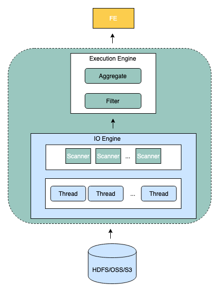
Backend is a backend node of StarRocks, which is responsible for data storage and SQL computing execution.
The BE nodes of StarRocks are corresponding to each other, and FE distributes data to the corresponding BE nodes according to certain policies. When data is imported, the data is directly written to BE nodes without being transferred through FE. BE is responsible for writing the imported data into the corresponding format and generating related indexes. When SQL computing is executed, an SQL statement is planned as a logical execution unit based on specific semantics. Then, it is split into specific physical execution units based on the distribution of data. These physical execution units are executed on the nodes of the data storage. This avoids data transmission and copying and achieves extreme query performance.
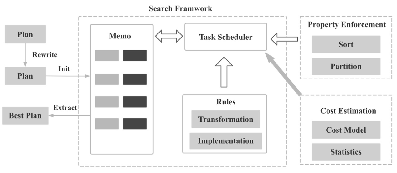
Generally, the more complex SQL statements, the more tables joined, and the larger the data volume, the more meaningful the query optimizer is. That happens because the performance of different execution methods may vary hundreds of times. The StarRocks optimizer is mainly implemented based on Cascades and ORCA papers and is deeply customized, optimized, and innovated in combination with the StarRocks executor and scheduler. The optimizer supports 99 SQL statements of TPC-DS and implements important features and optimization, such as common expression reuse, related subquery rewriting, Lateral Join, CTE reuse, Join Reorder, Join distributed execution strategy selection, Runtime Filter pushdown, and low-cardinality dictionary optimization.
One of the keys to determining the quality of the CBO is whether the Cost estimation is accurate, and one of the keys to the accuracy of the Cost estimation is whether the statistics are collected in a timely and accurate manner. StarRocks currently supports table-level and column-level statistics. It supports automatic and manual collecting methods that support full and sample collection methods.
MPP is short for massively parallel processing. Its core approach is to split a query plan into many compute instances that can be executed on a single node and then multiple nodes execute in parallel. Each node does not share CPU, memory, or disk resources. The query performance of an MPP database can continue to improve as the cluster expands horizontally.
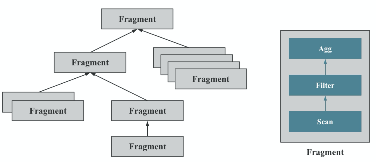
As shown in the preceding figure, StarRocks logically splits a query into multiple query fragments. Each query fragment can have one or more fragment execution instances. Each fragment execution instance is scheduled to be executed on a BE in the cluster. As shown in the preceding figure, a fragment can include one or more operators (execution operators). The fragment in the figure includes Scan, Filter, and Aggregate. As shown in the preceding figure, each fragment can have a different degree of parallelism.
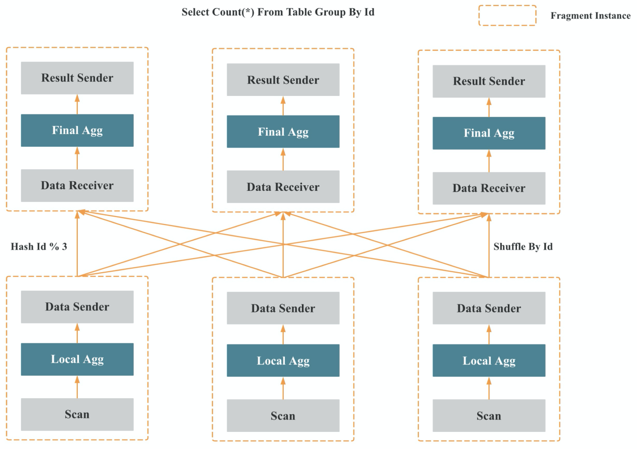
As shown in the preceding figure, multiple fragments are executed in parallel in memory in a pipeline manner instead of being executed stage by stage like a batch engine.
As shown in the preceding figure, the shuffle operation (data redistribution) is the key to the continuous improvement of the query performance of the MPP database with the horizontal expansion of the cluster. It is also the key to achieving high-cardinality aggregation and large table join.
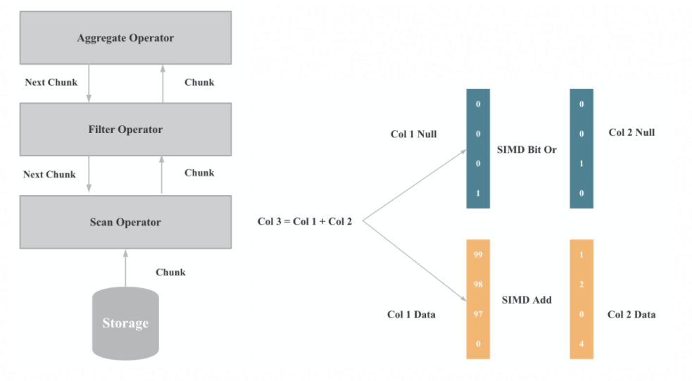
As the bottleneck of database execution gradually shifts from I/O to CPU, StarRocks re-implements the entire execution engine based on vectorization technology to give full play to the execution performance of the CPU. The core of the vectorized execution of operators and expressions is batch execution by column. Batch execution can have fewer virtual function calls and fewer branch judgments than single-row execution. Column-by-column execution is friendlier to the CPU and better for SIMD optimization than row-by-row execution.
Vectorized execution is the vectorization of all operators and expressions in the database and a huge and complex performance optimization project, including column organization of data on disks, memory, network, redesign of data structures and algorithms, memory management, and optimization of SIMD instruction, CPU Cache, and C++. Compared with the previous row-by-row execution, vectorized execution improves the overall performance by 5-10 times.
In the field of big data analytics, data is stored in data lakes in addition to data warehouses. Traditional implementation solutions of data lakes include Hive and HDFS. The concept of lake house has been popular in recent years. Common implementation solutions include Iceberg, Hudi, and Delta. Can StarRocks help users mine the value of data in data lakes? The answer is positive.
In the preceding content, we introduced how StarRocks implements blazing-fast analytics. If these capabilities are used in data lakes, they will lead to a better experience of data lake analytics. The next part will introduce how StarRocks implements blazing-fast data lake analytics.
Let's look at the overall architecture. The following figure shows the main modules related to StarRocks and data lake analytics. The data management is provided by data lakes, and the data storage is provided by Object Storage Services (such as Alibaba Cloud OSS and AWS S3) or by distributed file systems (such as HDFS).
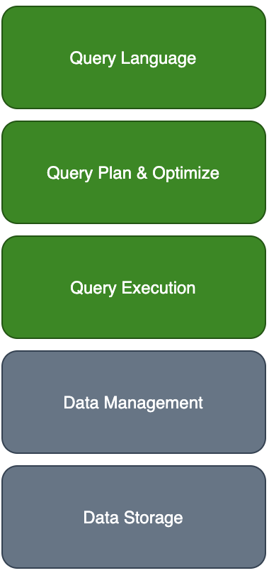
Currently, the capabilities for data lake analytics supported by StarRocks can be summarized in the following parts:
Next, let's look at how StarRocks endows data lakes with the capability for blazing-fast analytics in terms of query optimization and query execution.
This part of query optimization is mainly implemented using the CBO described earlier. The data lake module needs to give statistics to the optimizer. Based on those statistics, the optimizer uses a series of strategies to optimize query execution plans. Next, let's look at several common strategies through examples.
Let's take a look at the following example. In the generated execution plan, the HdfsScanNode contains statistics, such as cardunity and avgRowSize.
MySQL [hive_test]> explain select l_quantity from lineitem;
+-----------------------------+
| Explain String              |
+-----------------------------+
| PLAN FRAGMENT 0             |
|  OUTPUT EXPRS:5: l_quantity |
|   PARTITION: UNPARTITIONED  |
|                             |
|   RESULT SINK               |
|                             |
|   1:EXCHANGE                |
|                             |
| PLAN FRAGMENT 1             |
|  OUTPUT EXPRS:              |
|   PARTITION: RANDOM         |
|                             |
|   STREAM DATA SINK          |
|     EXCHANGE ID: 01         |
|     UNPARTITIONED           |
|                             |
|   0:HdfsScanNode            |
|      TABLE: lineitem        |
|      partitions=1/1         |
|      cardinality=126059930  |
|      avgRowSize=8.0         |
|      numNodes=0             |
+-----------------------------+
These statistics will be computed before officially entering the CBO. For example, we have MetaData Cache to cache these statistics for Hive, and we use manifest information of Iceberg to compute these statistics for Iceberg. After obtaining these statistics, the effect of the subsequent optimization strategy is improved.
Partition pruning is an optimization method that can only be performed when the destination table is a partition table. Partition pruning reduces the amount of computed data by analyzing the filter conditions in a query statement, only selecting partitions that may meet the conditions and not scanning partitions that do not match the conditions. For example, we created an external table with ss_sold_date_sk- as a partition column.
create external table store_sales(
      ss_sold_time_sk bigint
,     ss_item_sk bigint
,     ss_customer_sk bigint
,     ss_coupon_amt decimal(7,2)
,     ss_net_paid decimal(7,2)
,     ss_net_paid_inc_tax decimal(7,2)
,     ss_net_profit decimal(7,2)
,     ss_sold_date_sk bigint
) ENGINE=HIVE
PROPERTIES (
  "resource" = "hive_tpcds",
  "database" = "tpcds",
  "table" = "store_sales"
);
When the following query is executed, the data between partitions 2451911 and 2451941 will be read, and the data of other partitions will be filtered out, which can save a large part of network I/O consumption.
select ss_sold_time_sk from store_sales
where ss_sold_date_sk between 2451911 and 2451941
order ss_sold_time_sk; The query efficiency of joins of multiple tables has a strong correlation with the order in which each table participates. For example, there are two possible execution orders in the SQL statement select * from T0, T1, T2 where T0.a=T1.a and T2.a=T1.a:
According to the volume and distribution of data of T0 and T2, these two execution orders will have different performances. StarRocks implements the join reorder mechanism based on DP and greedy algorithms in the optimizer to solve this problem. Currently, data analytics for Hive supports Join Reorder. The support for other data sources is also under development. Here is an example:
MySQL [hive_test]> explain select * from T0, T1, T2 where T2.str=T0.str and T1.str=T0.str;
+----------------------------------------------+
| Explain String                               |
+----------------------------------------------+
| PLAN FRAGMENT 0                              |
|  OUTPUT EXPRS:1: str | 2: str | 3: str       |
|   PARTITION: UNPARTITIONED                   |
|   RESULT SINK                                |
|   8:EXCHANGE                                 |
| PLAN FRAGMENT 1                              |
|  OUTPUT EXPRS:                               |
|   PARTITION: HASH_PARTITIONED: 2: str        |
|   STREAM DATA SINK                           |
|     EXCHANGE ID: 08                          |
|     UNPARTITIONED                            |
|   7:HASH JOIN                                |
|   |  join op: INNER JOIN (BUCKET_SHUFFLE(S)) |
|   |  hash predicates:                        |
|   |  colocate: false, reason:                |
|   |  equal join conjunct: 1: str = 3: str    |
|   |----6:EXCHANGE                            |
|   4:HASH JOIN                                |
|   |  join op: INNER JOIN (PARTITIONED)       |
|   |  hash predicates:                        |
|   |  colocate: false, reason:                |
|   |  equal join conjunct: 2: str = 1: str    |
|   |----3:EXCHANGE                            |
|   1:EXCHANGE                                 |
| PLAN FRAGMENT 2                              |
|  OUTPUT EXPRS:                               |
|   PARTITION: RANDOM                          |
|   STREAM DATA SINK                           |
|     EXCHANGE ID: 06                          |
|     HASH_PARTITIONED: 3: str                 |
|   5:HdfsScanNode                             |
|      TABLE: T2                               |
|      partitions=1/1                          |
|      cardinality=1                           |
|      avgRowSize=16.0                         |
|      numNodes=0                              |
| PLAN FRAGMENT 3                              |
|  OUTPUT EXPRS:                               |
|   PARTITION: RANDOM                          |
|   STREAM DATA SINK                           |
|     EXCHANGE ID: 03                          |
|     HASH_PARTITIONED: 1: str                 |
|   2:HdfsScanNode                             |
|      TABLE: T0                               |
|      partitions=1/1                          |
|      cardinality=1                           |
|      avgRowSize=16.0                         |
|      numNodes=0                              |
| PLAN FRAGMENT 4                              |
|  OUTPUT EXPRS:                               |
|   PARTITION: RANDOM                          |
|   STREAM DATA SINK                           |
|     EXCHANGE ID: 01                          |
|     HASH_PARTITIONED: 2: str                 |
|   0:HdfsScanNode                             |
|      TABLE: T1                               |
|      partitions=1/1                          |
|      cardinality=1                           |
|      avgRowSize=16.0                         |
|      numNodes=0                              |
+----------------------------------------------+
Predicate pushdown pushes the computing of filtering expressions in query statements to the nearest place to a data source as much as possible, thus reducing the overhead of data transmission or computing. For data lake scenarios, we push filtering conditions, such as Min/Max, to the parquet, so the system can quickly filter out unused row groups when reading Parquet files.
For example, the condition corresponding to l_discount=1 is pushed down to the parquet side for the following query:
MySQL [hive_test]> explain select l_quantity from lineitem where l_discount=1;
+----------------------------------------------------+
| Explain String                                     |
+----------------------------------------------------+
| PLAN FRAGMENT 0                                    |
|  OUTPUT EXPRS:5: l_quantity                        |
|   PARTITION: UNPARTITIONED                         |
|                                                    |
|   RESULT SINK                                      |
|                                                    |
|   2:EXCHANGE                                       |
|                                                    |
| PLAN FRAGMENT 1                                    |
|  OUTPUT EXPRS:                                     |
|   PARTITION: RANDOM                                |
|                                                    |
|   STREAM DATA SINK                                 |
|     EXCHANGE ID: 02                                |
|     UNPARTITIONED                                  |
|                                                    |
|   1:Project                                        |
|   |  <slot 5> : 5: l_quantity                      |
|   |                                                |
|   0:HdfsScanNode                                   |
|      TABLE: lineitem                               |
|      NON-PARTITION PREDICATES: 7: l_discount = 1.0 |
|      partitions=1/1                                |
|      cardinality=63029965                          |
|      avgRowSize=16.0                               |
|      numNodes=0                                    |
+----------------------------------------------------+ In addition to the strategies mentioned above, we have adopted strategies, such as Limit pushdown, TopN pushdown, and subquery optimization, for data lake analytics. These strategies can help optimize query performance.
As mentioned earlier, the execution engine of StarRocks is omni-vectorized and of MPP architecture, which will bring great improvement to the data analytics in the data lake. Next, let's look at how StarRocks schedules and executes analytics queries of data lakes.
Data in a data lake is generally stored in HDFS and OSS, which meets the requirements in hybrid and non-hybrid deployment. We implement a set of load balancing algorithms for scheduling fragments.
After queries are scheduled to BEs for execution, the entire execution process is vectorized. Let's take a specific example of Iceberg. The corresponding BE of the IcebergScanNode is currently the vectorized implementation of HdfsScanNode. Other operators are similar and are the vectorized implementation at BEs.
MySQL [external_db_snappy_yuzhou]> explain select c_customer_id customer_id
    ->        ,c_first_name customer_first_name
    ->        ,c_last_name customer_last_name
    ->        ,c_preferred_cust_flag customer_preferred_cust_flag
    ->        ,c_birth_country customer_birth_country
    ->        ,c_login customer_login
    ->        ,c_email_address customer_email_address
    ->        ,d_year dyear
    ->        ,'s' sale_type
    ->  from customer, store_sales, date_dim
    ->  where c_customer_sk = ss_customer_sk
    ->    and ss_sold_date_sk = d_date_sk;
+------------------------------------------------
| PLAN FRAGMENT 0
|  OUTPUT EXPRS:2: c_customer_id | 9: c_first_name | 10: c_last_name | 11: c_preferred_cust_flag | 15: c_birth_country | 16: c_login | 17: c_email_address | 48: d_year | 70: expr |
|   PARTITION: UNPARTITIONED
|   RESULT SINK
|   9:EXCHANGE
| PLAN FRAGMENT 1
|  OUTPUT EXPRS:
|   PARTITION: RANDOM
|   STREAM DATA SINK
|     EXCHANGE ID: 09
|     UNPARTITIONED
|   8:Project
|   |  <slot 2> : 2: c_customer_id
|   |  <slot 9> : 9: c_first_name
|   |  <slot 10> : 10: c_last_name
|   |  <slot 11> : 11: c_preferred_cust_flag
|   |  <slot 15> : 15: c_birth_country
|   |  <slot 16> : 16: c_login
|   |  <slot 17> : 17: c_email_address
|   |  <slot 48> : 48: d_year
|   |  <slot 70> : 's'
|   7:HASH JOIN
|   |  join op: INNER JOIN (BROADCAST)
|   |  hash predicates:
|   |  colocate: false, reason:
|   |  equal join conjunct: 21: ss_customer_sk = 1: c_customer_sk
|   4:Project
|   |  <slot 21> : 21: ss_customer_sk
|   |  <slot 48> : 48: d_year
|   3:HASH JOIN
|   |  join op: INNER JOIN (BROADCAST)
|   |  hash predicates:
|   |  colocate: false, reason:
|   |  equal join conjunct: 41: ss_sold_date_sk = 42: d_date_sk
|   0:IcebergScanNode
|      TABLE: store_sales
|      cardinality=28800991
|      avgRowSize=1.4884362
|      numNodes=0
| PLAN FRAGMENT 2
|  OUTPUT EXPRS:
|   PARTITION: RANDOM
|   STREAM DATA SINK
|     EXCHANGE ID: 06
|     UNPARTITIONED
|   5:IcebergScanNode
|      TABLE: customer
|      cardinality=500000
|      avgRowSize=36.93911
|      numNodes=0
| PLAN FRAGMENT 3
|  OUTPUT EXPRS:
|   PARTITION: RANDOM
|   STREAM DATA SINK
|     EXCHANGE ID: 02
|     UNPARTITIONED
|   1:IcebergScanNode
|      TABLE: date_dim
|      cardinality=73049
|      avgRowSize=4.026941
| numNodes=0TPC-H is a test set developed by the Transaction Processing Performance Council (TPC) in the United States to simulate decision- and support-like applications. It consists of a suite of business-oriented ad-hoc queries and concurrent data modifications.
TPC-H models data according to real production environments to simulate the data warehouse of a sales system. The test consists of eight tables. The volume of data ranges from 1 GB to 3 TB. The benchmark test involves 22 query statements. The evaluation metrics mainly are the response time of each query, namely, the time required from submitting a query to receiving the result.
A comparative test is performed on a TPCH 100G-scale dataset with a total of 22 queries. The results are shown below:
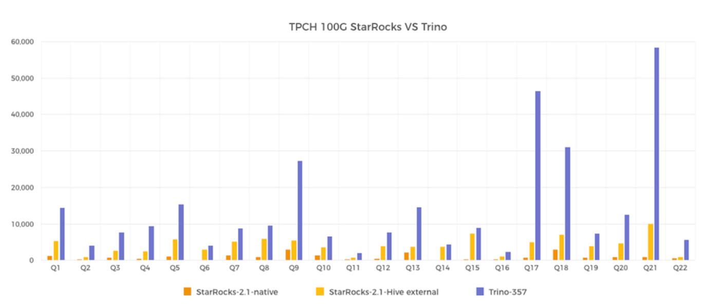
StarRocks uses local storage queries and Hive external table queries for testing. The StarRocks On Hive and Trino On Hive query the same data. The data is stored in ORC format and compressed in zlib format. The test environment is built through Alibaba Cloud EMR.
In the end, the StarRocks local storage query takes 21s, and the StarRocks Hive external table query takes 92s. The total Trino query time is 307s. StarRocks On Hive far exceeds Trino in query performance but is still a long way from Trino in terms of the local storage query. The main reason is that accessing remote storage increases network overhead, and the latency and IOPS of remote storage are usually not as good as those of local storage. The following plan is to make up for the problem through Cache and other mechanisms to help bridge the gap between StarRocks local tables and StarRocks On Hive.
Please refer to the comparison report of StarRocks vs. Trino TPCH performance test for the specific testing process (Article in Chinese).
Thanks to core technologies, such as omni-vectorized execution engine, CBO, and MPP execution architecture, StarRocks has achieved the capability for blazing-fast data lake analytics that far exceeds other similar products. In the long run, the vision of StarRocks of the data lake analytics is to provide simple, easy-to-use, and high-speed data lake analytics. StarRocks still has a lot of work to complete to achieve this goal, including:
[1] https://github.com/StarRocks/starrocks/issues/2772
[2] https://github.com/StarRocks/starrocks/issues/1030
[3] https://help.aliyun.com/document_detail/404790.html (Article in Chinese)
[4] StarRocks vs Trino TPCH Performance Testing comparison report (Article in Chinese)
New Features of Alibaba Cloud Remote Shuffle Service: AQE and Throttling

62 posts | 7 followers
FollowAlibaba EMR - April 21, 2022
Alibaba Cloud Big Data and AI - April 24, 2026
Apache Flink Community - April 30, 2024
Alibaba EMR - August 5, 2024
Alibaba Cloud Big Data and AI - April 15, 2026
Alibaba Cloud Big Data and AI - April 13, 2026

62 posts | 7 followers
Follow Big Data Consulting for Data Technology Solution
Alibaba Cloud provides big data consulting services to help enterprises leverage advanced data technology.
Learn More Big Data Consulting Services for Retail Solution
Alibaba Cloud experts provide retailers with a lightweight and customized big data consulting service to help you assess your big data maturity and plan your big data journey.
Learn More E-MapReduce Service
A Big Data service that uses Apache Hadoop and Spark to process and analyze data
Learn More Managed Service for Prometheus
Multi-source metrics are aggregated to monitor the status of your business and services in real time.
Learn MoreMore Posts by Alibaba EMR