Integration of Paimon and Spark - Part 2: Query Optimization

Through a series of optimizations, we have improved the performance of Paimon × Spark on TpcDS by over 37%, which is basically the same as that of Parquet × Spark. This article describes the key optimization points in detail.

Paimon

Apache Paimon (incubating) is a streaming data lake storage technology that provides users with high-throughput, low-latency data ingestion, streaming subscription, and real-time query capabilities. Paimon uses open data formats and technology concepts to connect with mainstream computing engines in the industry, such as Flink, Spark, and Trino, to promote the popularization and development of the streaming lakehouse architecture.

Paimon × Spark

Apache Spark, as a unified computing and analysis engine for big data processing, not only supports high-level APIs in multiple languages, but also a wide range of big data scenario applications, including Spark SQL for structured data processing, MLlib for machine learning, GraphX for graph processing, and Structured Streaming for incremental computing and stream processing. Spark has become an essential part of the big data software stack. For Paimon to land more conveniently in quasi-real-time and offline lake warehouse scenarios, deep and comprehensive integration with Spark is imperative.

In the previous Paimon release, we focused on the integration of Paimon's features with the Spark SQL ecosystem, including Schema Evolution, Structured Streaming Read/Write, Dynamic Insert Overwrite Partition, Update/Merge Into, and so on. In the recent release of 0.6 and 0.7, we started to work on Paimon's performance based on Spark SQL queries. Initially, we will combine the existing optimization rules and frameworks of Spark SQL to make full use of these. Through a series of optimizations, we have improved the performance of Paimon × Spark on TpcDS by over 37%, which is similar to that of Parquet × Spark. The following text provides a detailed introduction to the key optimization points.

Dynamic Partition Pruning

Dynamic partition pruning (DPP) is a common optimization point in SQL optimization. It is essentially an extension of predicate pushdown. Its purpose is to minimize the I/O cost of reading data from the data source and reduce the computing cost.

In a data warehouse, a large fact table and a small dimension table are often associated for query, and the fact table needs to be filtered based on the field information in the dimension table, as shown in the following SQL code snippet in TpcDS Q14:

select ss_quantity quantity ,ss_list_price list_ price
from store_sales, date_dim
where ss_sold_date_sk = d_date_sk and d_year between 1999 and 1999 + 2
order by quantity limit 10;

The execution plan in the case where DPP is not supported is simplified as follows:

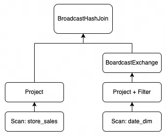
Paimon applies the Spark DataSource V2 query framework, which provides SupportsRuntimeFiltering interfaces for V2 tables to implement run-time dynamic filtering after Spark3.2. Theoretically, the filter conditions of any field (including common data fields and partition fields) can be applied, but in general, only the filter conditions of partition fields can be fully applied, that is, filter nodes at upper layers are not needed to filter and select data. Paimon tables use this interface to implement dynamic partition pruning. The execution plan after DPP is supported is as follows:

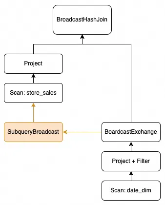
Under the TpcDS data set of 1 TB, the amount of data in store_sales table which participate in the join is reduced from 2.7 billion to 1.6 billion after DPP is applied. After only this optimization is applied, Q14 running time is reduced to about 55% of the original time, and the query performance of the 1 TB TpcDS data set is improved by over 20%;

Related code:

Exchange Reuse

Exchange is a key operation in the physical plan of Spark, which corresponds to the shuffle in the logical plan. In the execution phase, exchange can represent the data output by some plans in an SQL statement. In complex SQL, we can define an SQL code snippet through the common table expression (CTE) syntax, which can be used to simplify the entire SQL or be used multiple times. Take the following simplified TpcDS Q23 as an example. One of the defined CTE frequent_ss_items is used twice throughout the SQL.

with frequent_ss_items as (
  select substr(i_item_desc,1,30) itemdesc, i_item_sk item_sk, d_date solddate, count(*) cnt
  from store_sales, date_dim, item
  where ss_sold_date_sk = d_date_sk and ss_item_sk = i_item_sk and d_year in (2000,2000+1,2000+2,2000+3)
  group by substr(i_item_desc,1,30),i_item_sk,d_date
  having count(*) >4
),
max_store_sales as (...),
best_ss_customer as (...)
select sum(sales)
from (
  select cs_quantity*cs_list_price sales
       from catalog_sales
           ,date_dim
       where d_year = 2000
         and d_moy = 2
         and cs_sold_date_sk = d_date_sk
         and cs_item_sk in (select item_sk from frequent_ss_items)
         and cs_bill_customer_sk in (select c_customer_sk from best_ss_customer)
      union all
      select ws_quantity*ws_list_price sales
       from web_sales
           ,date_dim
       where d_year = 2000
         and d_moy = 2
         and ws_sold_date_sk = d_date_sk
         and ws_item_sk in (select item_sk from frequent_ss_items)
         and ws_bill_customer_sk in (select c_customer_sk from best_ss_customer)
) y
limit 100;

Obviously, in the execution phase, we want the frequent_ss_items to be executed only once, and the executed data can be cached, and then the subsequent catalog_sales and web_sales table join operations are performed respectively. For this scenario, Spark provides exchange reuse optimization. The expected execution plan is simplified as follows:

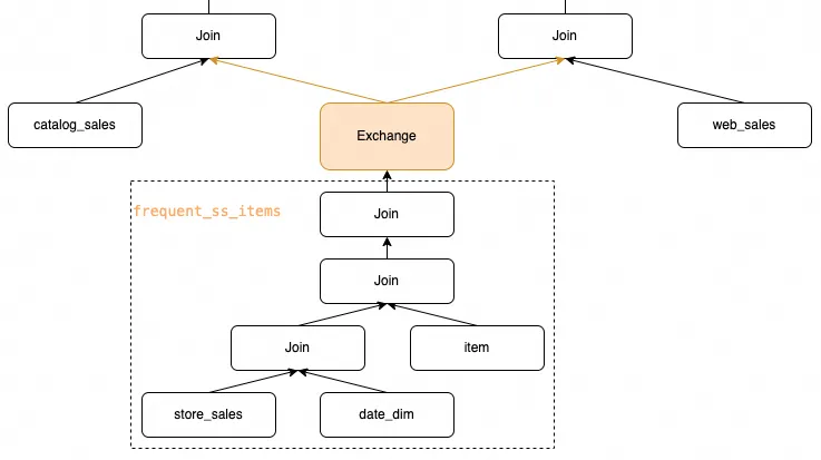
However, this optimization relies on the hashCode of each physical operation in the operator plan to determine whether the actual runtime can be reused. We have located and solved the implementation problems in Paimon, so that Paimon can use the optimization of exchange reuse provided by Spark, thus reducing unnecessary redundant computing and reducing I/O and network overhead. After only this optimization is applied, Q23 running time is reduced to about 50% of the original time, and the query performance of the 1 TB TpcDS data set is improved by over 13%.

Dynamic Adjustment of Scan Concurrency

Concurrency during the actual execution of a task is one of the key factors influencing the performance of a job. Spark provides spark.sql.shuffle.partitions parameters to adjust the concurrency of operators such as Join or Agg, and also provides the adaptive query execution (AQE) framework to dynamically adjust the concurrency, but these cannot affect the concurrency of the scan phase of reading data sources.

Under the framework of DataSource V2, the scan mode of the data source, including concurrency, is completely determined by the DataSource itself. Let's take TpcDS Q19 as an example:

select  i_brand_id brand_id, i_brand brand, i_manufact_id, i_manufact,
    sum(ss_ext_sales_price) ext_price
 from date_dim, store_sales, item,customer,customer_address,store
 where d_date_sk = ss_sold_date_sk
   and ss_item_sk = i_item_sk
   and i_manager_id=8
   and d_moy=11
   and d_year=1998
   and ss_customer_sk = c_customer_sk 
   and c_current_addr_sk = ca_address_sk
   and substr(ca_zip,1,5) <> substr(s_zip,1,5) 
   and ss_store_sk = s_store_sk 
 group by i_brand
      ,i_brand_id
      ,i_manufact_id
      ,i_manufact
 order by ext_price desc
         ,i_brand
         ,i_brand_id
         ,i_manufact_id
         ,i_manufact
limit 100 ;

Its customer_address and store are joined based on the condition substr(ca_zip,1,5) <> substr(s_zip,1,5).

If CBO is not introduced to reorder the join, the two tables are implemented by BroadcastNestedLoopJoin, and exchange is not introduced to adjust the concurrency of the join. The following figure shows the execution plan:

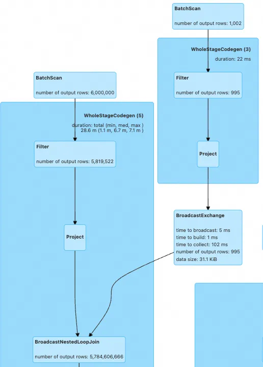
Before the introduction of optimization, the overall execution performance was poor because the data shards of the customer_address table were small, but the task computing load was high (serious expansion after data joining).

In response to this problem, Paimon provides the ability to dynamically adjust the data shards of the data source based on the number of available cores of the current job, and further adjust the concurrency to improve the query efficiency.

After only this optimization is applied, Q19 running time is reduced to about 25% of the original time, and the query performance of the 1 TB TpcDS data set is improved by over 14%.

Merge Scalar Subqueries

Similar to exchange reuse, merge scalar subquery optimization traverses the entire SQL logical execution plan to extract scalar subqueries, and attempts to merge multiple scalar subqueries so that multiple scalar values are obtained by executing the subqueries only once.

Let's take the code snippet of TpcDS Q9 as an example. The whole Q9 consists of five case-when statements.

select case when (select count(*) 
                  from store_sales 
                  where ss_quantity between 1 and 20) > 74129
            then (select avg(ss_ext_discount_amt) 
                  from store_sales 
                  where ss_quantity between 1 and 20) 
            else (select avg(ss_net_paid)
                  from store_sales
                  where ss_quantity between 1 and 20) end bucket1
from reason
where r_reason_sk = 1;

In this SQL code, the three parts: the case-when condition, THEN, and ELSE statements use the same filter condition to read the same table, and only the aggregate expression is different. Without this optimization, the execution plan is as follows:

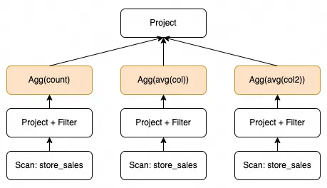
Spark itself provides MergeScalarSubQueries optimization rules, but it cannot be better implemented to connect to DataSource V2 tables like Paimon. Therefore, we implement it separately on the Paimon side and inject Paimon's self-implemented optimization into the Spark optimizer through the Extensions interface provided by Spark. After the optimization is applied, the execution plan is as follows:

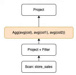
Therefore, the query optimization of merging scalar subqueries effectively reduces redundant computing and improves the query performance of Paimon in this scenario. After only applying this optimization, the Q9 running time is reduced to 57% of the original time.

Cost-Based Optimization

Spark SQL allows you to use a cost-based optimizer (CBO) to improve query performance, mainly for multi-join scenarios, using dynamic planning algorithms to select the join order with the lowest cost. A more effective optimization depends on the cost calculation model and the collection of table-level and column-level statistics of the table, and the column-level statistics are particularly important in evaluating the runtime statistics of the Plan operator node.

The new version of Paimon adds statistical information to metadata, which can be collected through the native Spark Analyze command and connected to Spark SQL so that Spark SQL can use Paimon table-level or column-level information for query optimization. Let's take TpcDS Q24a as an example:

with ssales as
(select c_last_name, c_first_name, s_store_name, ca_state, s_state, i_color, i_current_price, i_manager_id, i_units, i_size, sum(ss_net_paid) netpaid
from store_sales, store_returns, store, item, customer, customer_address
where ss_ticket_number = sr_ticket_number
  and ss_item_sk = sr_item_sk
  and ss_customer_sk = c_customer_sk
  and ss_item_sk = i_item_sk
  and ss_store_sk = s_store_sk
  and c_current_addr_sk = ca_address_sk
  and c_birth_country <> upper(ca_country)
  and s_zip = ca_zip
and s_market_id=8
group by c_last_name, c_first_name, s_store_name, ca_state, s_state, i_color, i_current_price, i_manager_id, i_units, i_size)
select c_last_name, c_first_name, s_store_name, sum(netpaid) paid
from ssales
where i_color = 'peach'
group by c_last_name, c_first_name, s_store_name
having sum(netpaid) > (select 0.05 * avg(netpaid) from ssales)
order by c_last_name, c_first_name, s_store_name;

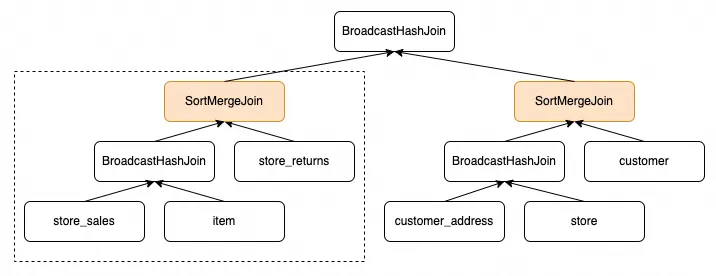
The following figure shows the execution plan for the ssales part of the CTE. The two SortMergeJoin operations are included. The left-side dotted line box shows join operations between large amounts of data, which seriously affects the performance.

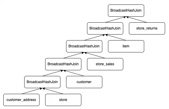
The following figure shows the execution plan after you execute the Analyze statement to provide the column-level statistics. The tables that participate in the Join statement are reordered and all Join statements are executed in the BroadcastHashJoin manner.

Paimon provides complete statistics. With the help of the CBO framework, not only can the corresponding query performance be improved, but SQL that cannot run under normal resource configuration can also run normally, such as TpcDS Q72. After the optimization is superimposed on the previous optimization items, Q24 running time is reduced to about 23% of the original time, and the overall query performance of the 1 TB TpcDS data set is improved to about 30%.

Related code:

Optimization effects

In this topic, the EMR 5.16.0 version of Alibaba Cloud is used. The following table describes the attributes of cluster nodes.

master: 1 * ecs.g7.8xlarge 32 vCPU 128 GiB
core: 6 * ecs.g7.8xlarge 32 vCPU 128 GiB

The following components and versions are used:

Paimon: 0.8-SNAPSHOT (corresponding to commit: 193df7345aa520f8b45125cdd85588a91a3fc3a9)
Spark: 3.3.1 (additional cherry-pick SPARK-41378 to support stats-related functions in DataSource V2)

Spark-related configurations enabled:

spark.executor.cores	4
spark.executor.memory	14g
spark.executor.memoryOverhead	2g
spark.dynamicAllocation.enabled	true
spark.sql.cbo.enabled	true
spark.sql.cbo.joinReorder.enabled	true
spark.sql.autoBroadcastJoinThreshold	128m

The Paimon table uses the append table (no primary key table), uses parquet as the file format, and sets bucket=-1 (the latest code has the default setting: PAIMON-2829), which facilitates comparison with the Spark parquet table.

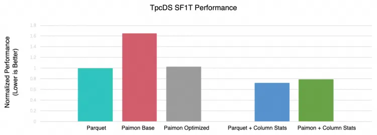
The preceding figure shows that we use the parquet table (with table-level statistics, that is, rowCount and sizeInByte) as the benchmark, which is used to compare the performance of the Paimon table (with table statistics only) before and after these optimizations to the right, and the query performance of the Parquet table and Paimon table when column-level statistics are collected.

The comparison shows that the optimized Paimon and Parquet basically have the same performance in normal cases (without column-level statistics). After column-level statistics are enabled, Paimon is about 8% slower than Parquet. This gap will also be one of the directions for performance optimization that we will continue to follow.

Follow-up Planning

In the lakehouse system, we believe that optimizing read/write queries will always be a long-term task. The current optimization efforts are primarily aimed at enabling Paimon to fully leverage the existing optimization rules or frameworks of Spark SQL. As we continue to progress, we will also utilize Paimon's own features, such as index or clustering, to optimize scan and further enhance Paimon's performance.

In addition, many tables without primary keys are still used in the current lakehouse scenarios, and the upsert capability for append tables is also one of the important plans for the future.

Community

Integration of Paimon and Spark - Part 2: Query Optimization

Paimon

Paimon × Spark

Dynamic Partition Pruning

Exchange Reuse

Dynamic Adjustment of Scan Concurrency

Merge Scalar Subqueries

Cost-Based Optimization

Optimization effects

Follow-up Planning

Read previous post:

Read next post:

Alibaba EMR

You may also like

Comments

Alibaba EMR

Related Products

Big Data Consulting for Data Technology Solution

Big Data Consulting Services for Retail Solution

ApsaraDB for HBase

Financial Services Solutions