Overview
A relational model's computation logic follows two key principles:
-
Only the fields in the current query and associated fields are used in the computation. (If a query contains fields from only one logical table, other logical tables in the relational model are not included in the computation.)
-
The model preserves the integrity of measure field data.
This diagram shows the general processing flow. Compared to direct physical joins, the relational model effectively prevents data expansion:

This overview simplifies the relational model's processing logic. In practice, factors such as cardinality, data match rates, and field types trigger different processing methods. See the following examples for details.
Examples
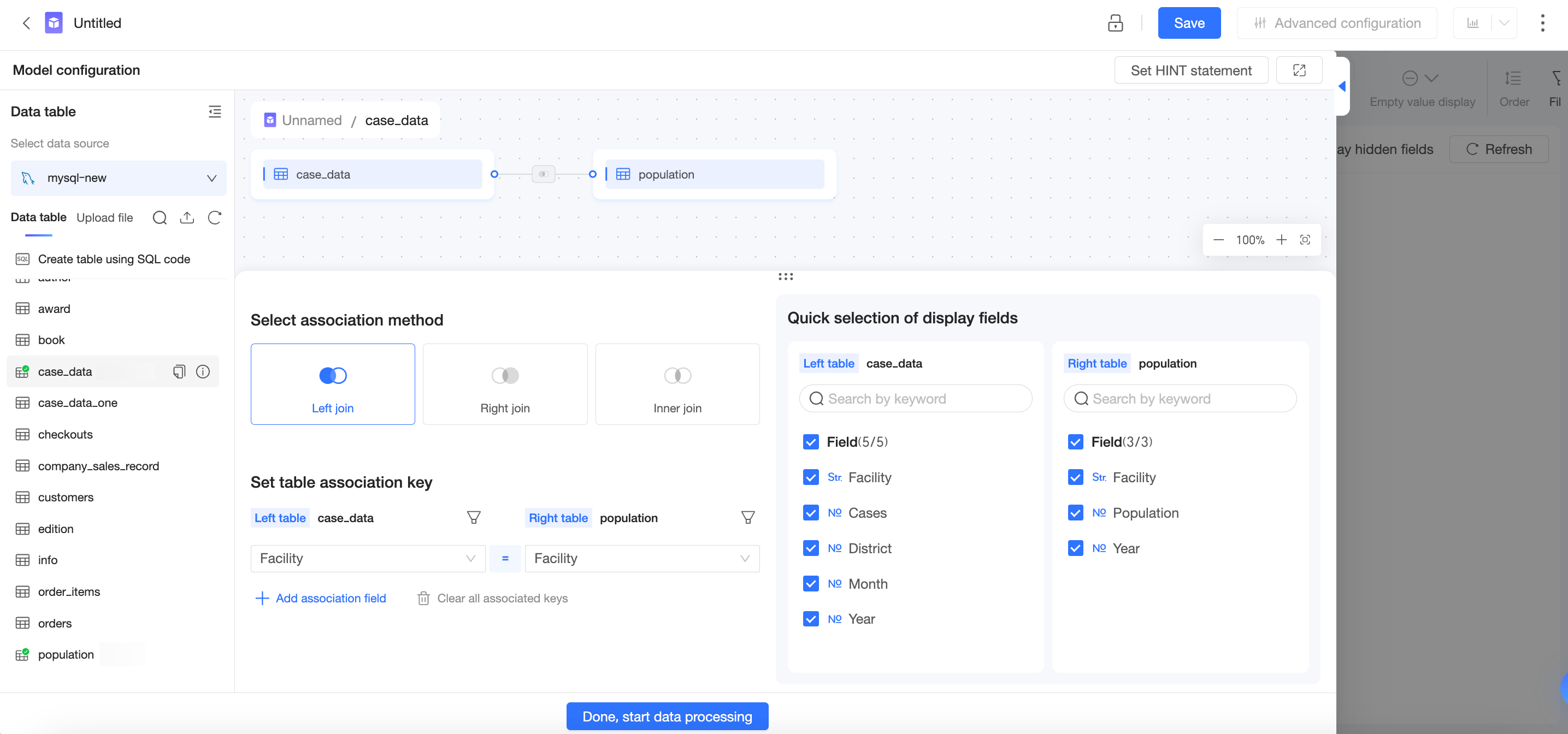
Model configuration
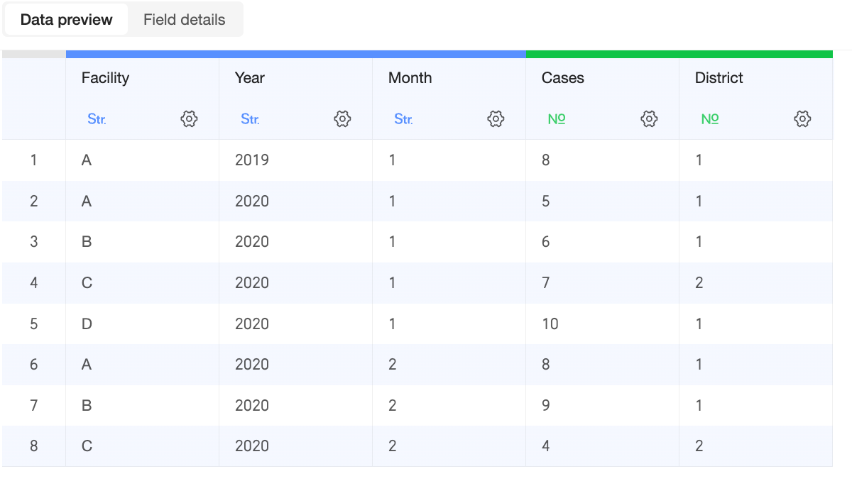
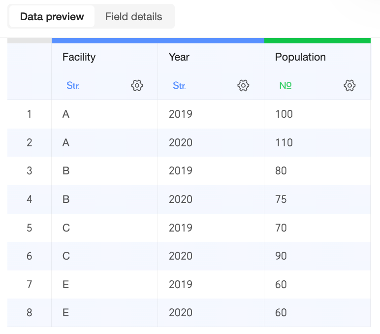
Data table fields
|
Primary table: Cases |
Secondary table: Population |
|
|
|
Relational model structure
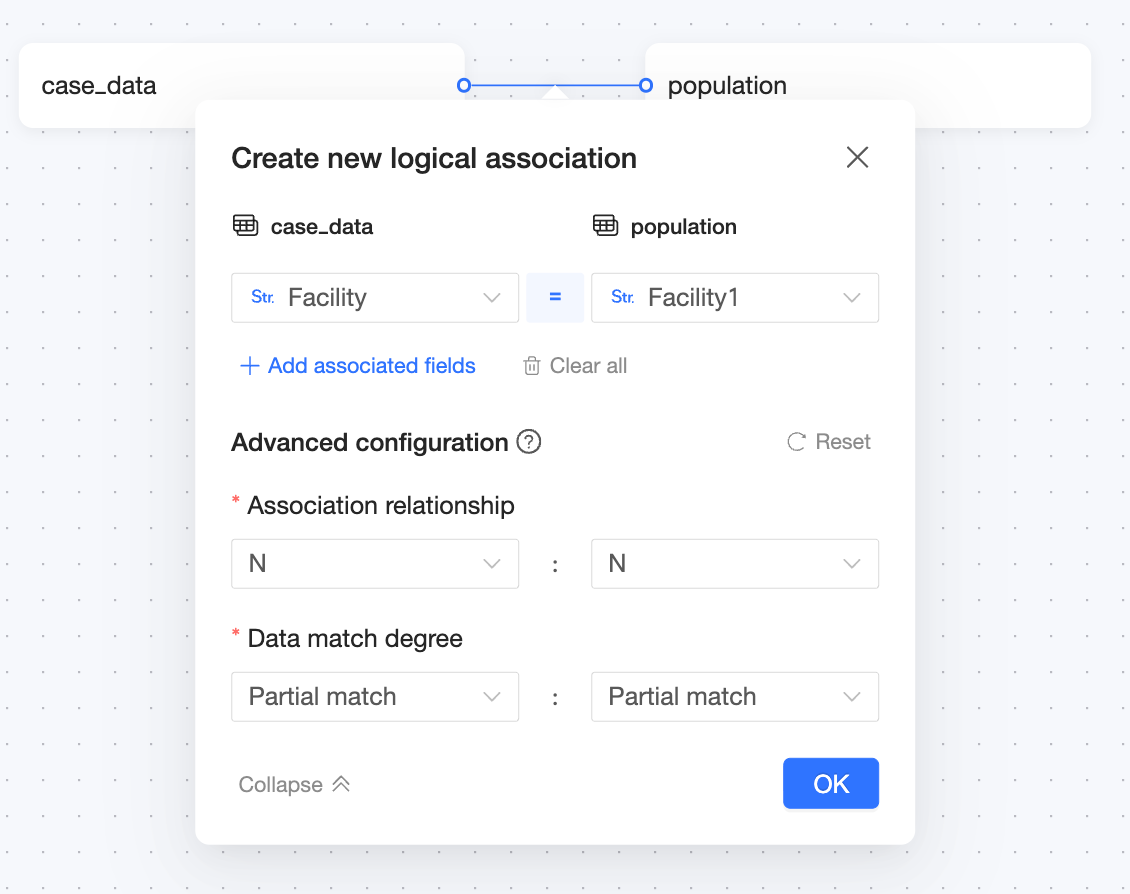
Where:
-
Join key: Medical Institution = Medical Institution
-
Join relationship: N:N
-
Data match rate: Partial Match: Partial Match
Chart configuration and calculation methods
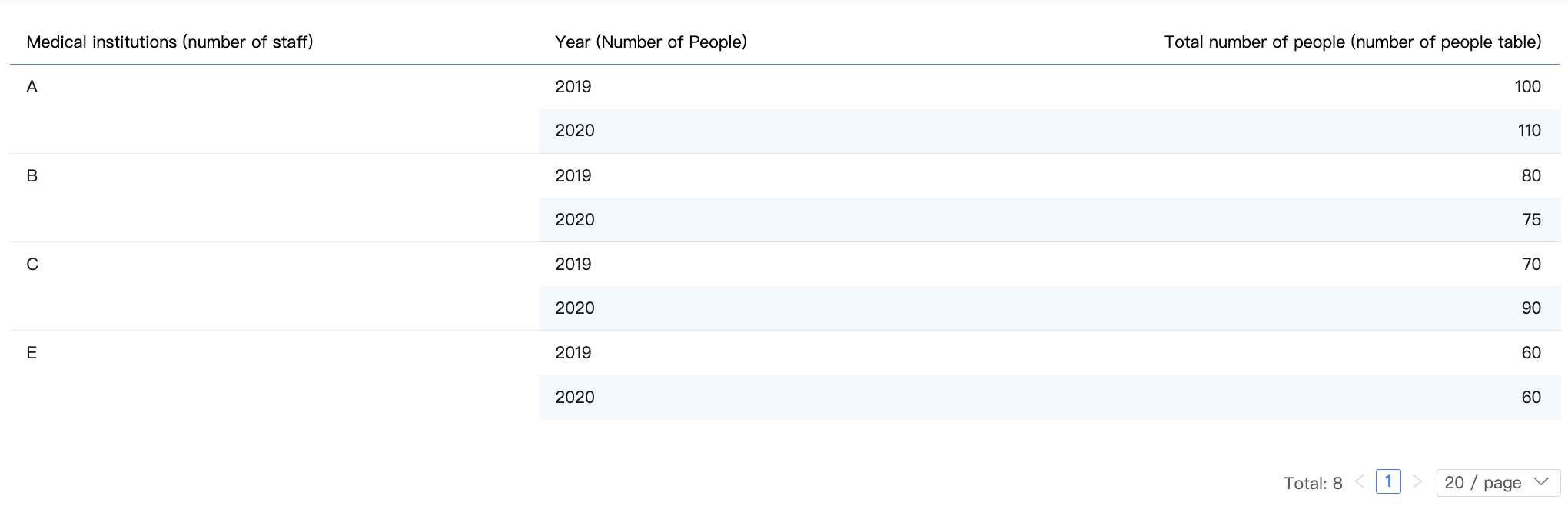
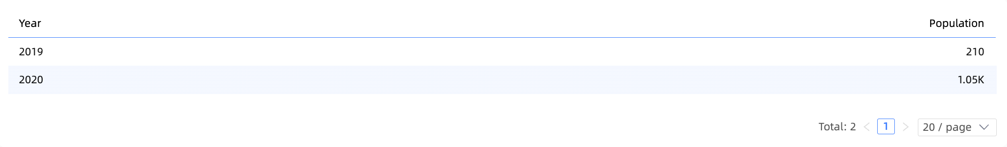
Single-table query
Chart configuration
|
Dimension |
Medical Institution (Population table), Year (Population table) |
|
Measure |
Sum of Population (Population table) |
Result data
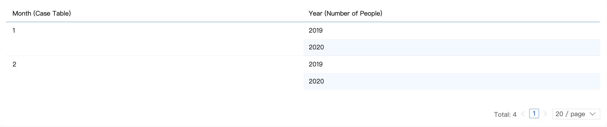
Multi-table query (dimensions only)
Chart configuration
|
Dimension |
Month (Cases table), Year (Population table) |
|
Measure |
- |
Result data
Inner join logic
-
Using an
INNER JOIN: When a chart contains only dimensions, only matched data is considered meaningful. Unmatched data, such as for medical institutions D and E, is ignored. -
The system joins the two tables on the "Medical Institution" field using an
INNER JOINto create an intermediate table. After deduplication, the system displays the result data.Institution (Cases)
Month (Cases)
Institution (Population)
Year (Population)
A
1
A
2020
A
1
A
2019
B
1
B
2020
B
1
B
2019
C
1
C
2020
C
1
C
2019
A
2
A
2020
A
2
A
2019
B
2
B
2020
B
2
B
2019
C
2
C
2020
C
2
C
2019
A
1
A
2020
A
1
A
2019
Multi-table query (measures only)
Chart configuration
|
Dimension |
- |
|
Measure |
Sum of Number of Cases (Cases table), Sum of Population (Population table) |
Result data

Calculation logic
-
When a query contains only measures and no dimensions, the aggregation produces a single row of data.
-
In this scenario, the system aggregates the measures from the
Cases tableandPopulation tableseparately and then appends the results.
Multi-table query (dimensions and measures)
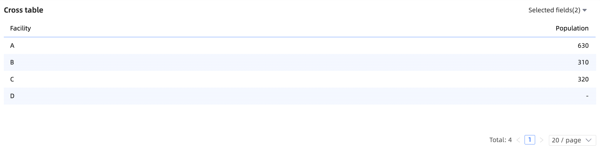
Example 1: Left table dimension, right table measure
Chart configuration
|
Dimension |
Medical Institution (Cases table) |
|
Measure |
Sum of Population (Population table) |
Result data
Calculation steps
Step 1: The dimension combination is computed from the dimension field in the chart, Medical Institution (Cases table), and the join key from the measure's table, Medical Institution (Population table).
Because this query includes a measure from the Population table, this step preserves all dimension values from that table. This ensures the integrity of the measure during subsequent calculations.
|
Institution (Population) |
Institution (Cases) |
|
A |
A |
|
B |
B |
|
C |
C |
|
E |
- |
Step 2: The dimension combination is then joined with the Population table to create an intermediate table. Since only the dimension combination is joined and each medical institution is unique within it, no data explosion occurs.
|
Institution (Population) |
Institution (Cases) |
Population (Population) |
|
A |
A |
100 |
|
B |
B |
80 |
|
C |
C |
70 |
|
A |
A |
110 |
|
B |
B |
75 |
|
C |
C |
90 |
|
- |
E |
60 |
|
- |
E |
60 |
Step 3: Aggregate the intermediate table by the dimension used in the chart to get the final result.
Because "Medical Institution E" from the Population table could not be matched with an entry in the Cases table, the result contains a row where the Medical Institution dimension is a null value.
Example 2: Left table dimension, right table measure (incorrect)
Chart configuration
|
Dimension |
Year (Cases table) |
|
Measure |
Sum of Population (Population table) |
Result data
Calculation steps
Step 1: The dimension combination is computed from the dimension field in the chart, Year (Cases table), and the join key from the measure's table, Medical Institution (Population table). For clarity, Medical Institution (Cases table) is also shown here.
Because this query includes a measure from the Population table, this step preserves all dimension values from that table. This ensures the integrity of the measure during subsequent calculations.
|
Institution (Population) |
Institution (Cases) |
Year (Cases) |
|
A |
A |
2019 |
|
A |
A |
2020 |
|
B |
B |
2020 |
|
C |
C |
2020 |
|
E |
- |
- |
In the Cases table, "Medical Institution A" has records for both 2019 and 2020. As a result, the dimension combination contains two rows for "A" in the Medical Institution (Population table) field.
Step 2: The dimension combination is then joined with the Population table to create an intermediate table.
|
Year (Cases) |
Institution (Population) |
Population (Population) |
|
2019 |
A |
100 |
|
2020 |
A |
100 |
|
2020 |
B |
80 |
|
2020 |
C |
70 |
|
2019 |
A |
110 |
|
2020 |
A |
110 |
|
2020 |
B |
75 |
|
2020 |
C |
90 |
|
- |
E |
60 |
|
- |
E |
60 |
Joining the two duplicate "A" rows in the dimension combination to the Population table duplicates the population data for "Medical Institution A", causing a data explosion.
Step 3: The intermediate table is then aggregated by the dimension used in the chart to produce the final result.
In this scenario, a data explosion occurs even when using a relational model. To avoid such issues, we recommend the following:
-
Configure join keys correctly: In this example, you should set both
Medical InstitutionandYearas a composite join key. This prevents data explosion when the intermediate table is generated in Step 2. -
Use dimensions and measures from the same logical table when cross-table queries are not needed: In this example, querying
Medical InstitutionandPopulationfrom just thePopulation tablewill produce the correct results.
Example 3: Right table dimension, left table measure (incorrect)
Chart configuration
|
Dimension |
Year (Population table) |
|
Measure |
Sum of Number of Covered Areas (Cases table) |
Result data
Calculation steps
Step 1: The dimension combination is computed from the dimension field in the chart, Year (Population table), and the join key from the measure's table, Medical Institution (Cases table). For clarity, Medical Institution (Population table) is also shown here.
Because this query includes a measure from the Cases table, this step preserves all dimension values from that table. This ensures the integrity of the measure during subsequent calculations.
|
Institution (Cases) |
Institution (Population) |
Year (Population) |
|
A |
A |
2020 |
|
A |
A |
2019 |
|
B |
B |
2020 |
|
B |
B |
2019 |
|
C |
C |
2020 |
|
C |
C |
2019 |
|
D |
- |
- |
In the Population table, medical institutions A, B, and C each have records for both 2019 and 2020. This causes two rows for "A", two for "B", and two for "C" to appear in the dimension combination in the Medical Institution (Cases table) field. Medical Institution E from the population table is not matched.
Step 2: The dimension combination is then joined with the Cases table to create an intermediate table.
|
Institution (Cases) |
Year (Population) |
Covered areas (Cases) |
|
A |
2020 |
1 |
|
A |
2019 |
1 |
|
B |
2020 |
1 |
|
B |
2019 |
1 |
|
C |
2020 |
2 |
|
C |
2019 |
2 |
|
A |
2020 |
1 |
|
A |
2019 |
1 |
|
B |
2020 |
1 |
|
B |
2019 |
1 |
|
C |
2020 |
2 |
|
C |
2019 |
2 |
|
D |
- |
1 |
|
A |
2020 |
1 |
|
A |
2019 |
1 |
Joining the duplicate rows for medical institutions A, B, and C in the dimension combination to the Cases table duplicates the Number of Covered Areas data, causing a data explosion.
Step 3: The intermediate table is then aggregated by the dimension used in the chart to produce the final result.
This query incorrectly calculates the sum of Number of Covered Areas for medical institutions A, B, and C due to duplication. The cause and recommendations are the same as in Example 2.
-
Configure join keys correctly: You should set
Medical InstitutionandYearas a composite join key. -
Use dimensions and measures from the same logical table when cross-table queries are not needed: You should query
YearandNumber of Covered Areasfrom just theCases table.
Comparison with physical modeling
In previous versions, Quick BI used physical modeling for datasets. This approach provides a visual interface to configure joins and merge multiple tables into a single wide table.
With physical modeling, you must explicitly define the join type, such as left join, inner join, or full join. This requires you to thoroughly understand your data and preprocess it for integrity and uniqueness. Otherwise, you risk severe issues such as data explosion.
A detailed example
Model configuration
Data table fields
|
Cases table |
Population table |
|
|
|
Physical model structure
Physical model wide table
Because the 'Medical Institution' field contains non-unique values, a severe data explosion occurs after physical modeling. For example, in the figure below, the 'Population (Population table)' for 'Medical Institution' 'A' and 'Year (Population table)' '2019' is incorrectly counted three times.
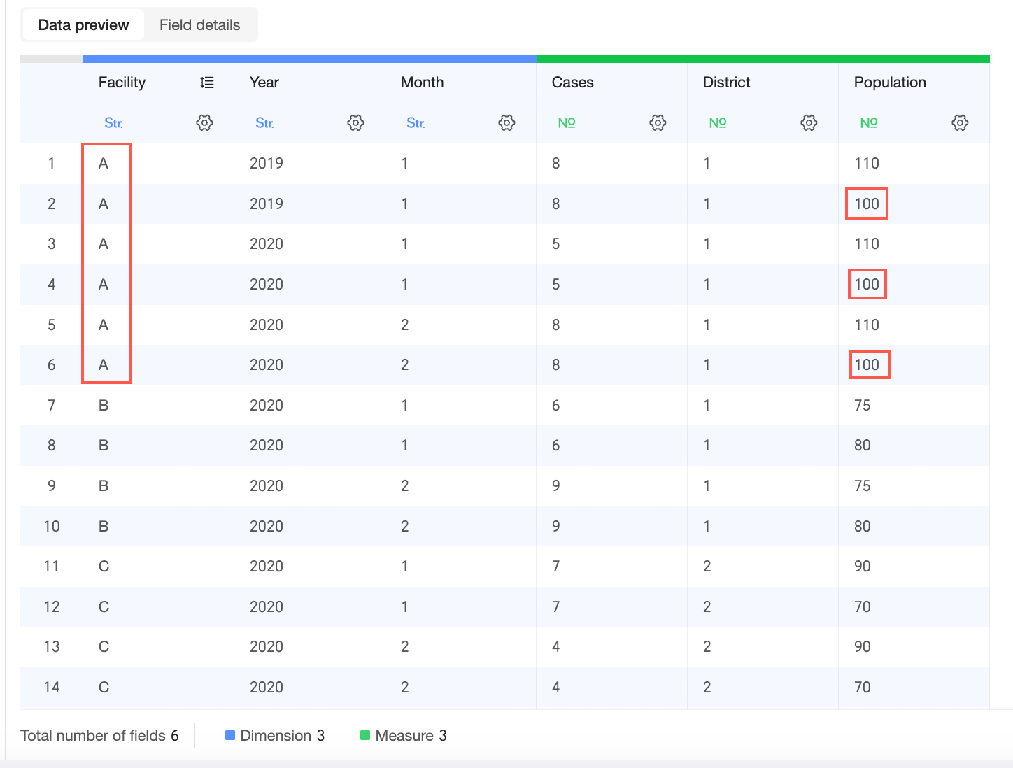
Chart configuration and calculation
Example 1
Chart configuration
|
Dimension |
Medical Institution (Cases table) |
|
Measure |
Sum of Population (Population table) |
Result data
Correct result
Example 2
Chart configuration
|
Dimension |
Year (Cases table) |
|
Measure |
Sum of Population (Population table) |
Result data
Correct result
Drawbacks of physical modeling
With physical modeling, you must validate the model's accuracy. When data contains non-unique values or is missing, you must take extra steps to prevent data errors, such as:
-
Use SQL to aggregate non-unique data before creating a join.
-
Use an LOD function to specify the aggregation granularity and prevent incorrect calculations.
-
Use SQL to supplement missing data or adjust the join type to account for data gaps and prevent data loss.
These operations require SQL expertise, making them difficult for non-technical business users. The physical modeling process is also tedious and complex, requiring repeated result verification.
In physical modeling, joining more tables increases the risk of data explosion and makes troubleshooting difficult. To minimize joins, you typically create a separate model for each analysis scenario. However, this leads to dataset proliferation as scenarios increase, making governance and maintenance harder over time.
Relational model: special cases
Handling cross-table fields
A cross-table field is a calculated field that uses fields from multiple logical tables. It does not belong to any single logical table and is categorized separately in the dataset.
Cross-table field calculations always involve multiple logical tables, and the result depends on their join relationships as determined by the query's measures and dimensions. Because of this dependency, these fields can only be computed in a specific query context, and their detail-level data is unavailable for preview.
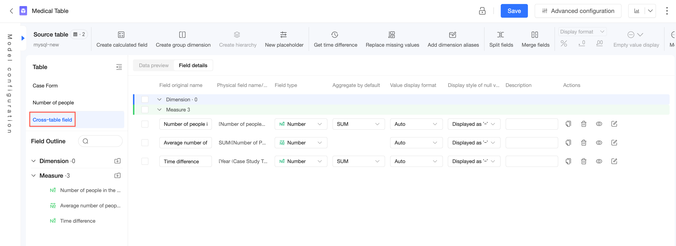
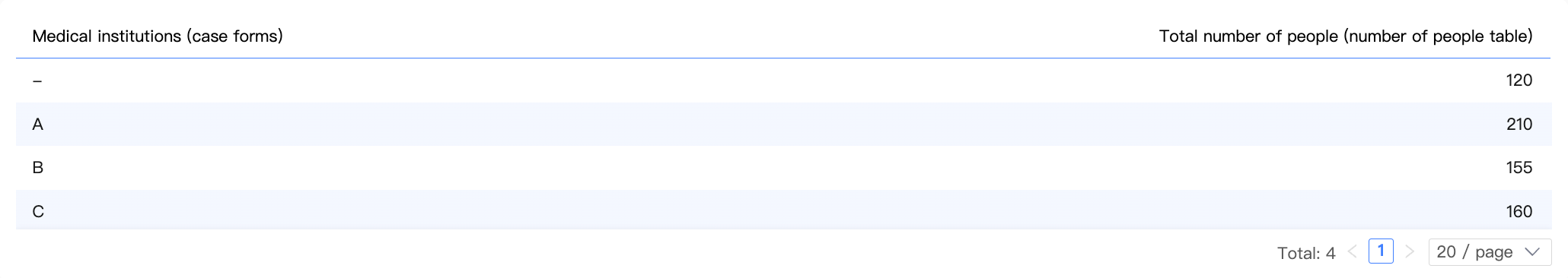
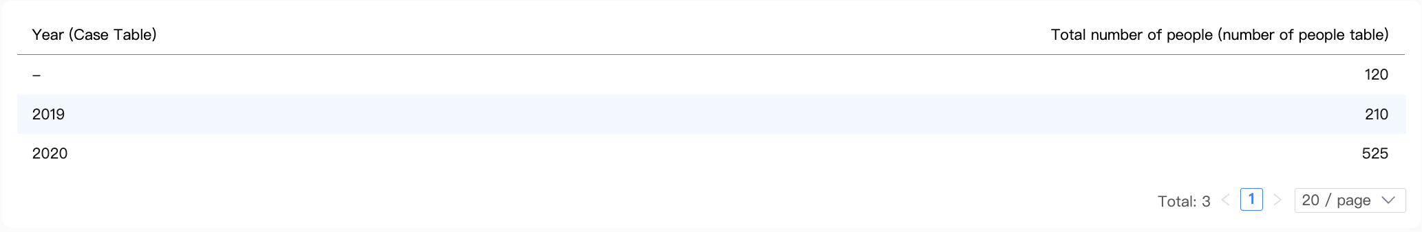
Post-aggregation cross-table fields
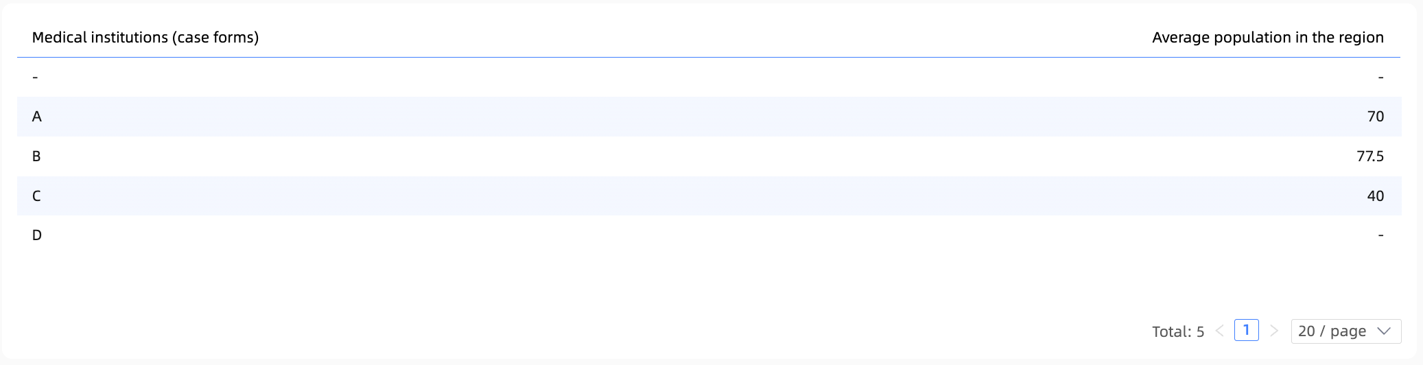
You create a post-aggregation cross-table field by first aggregating fields from single tables, then using them in a cross-table arithmetic calculation (such as addition, subtraction, multiplication, or division).
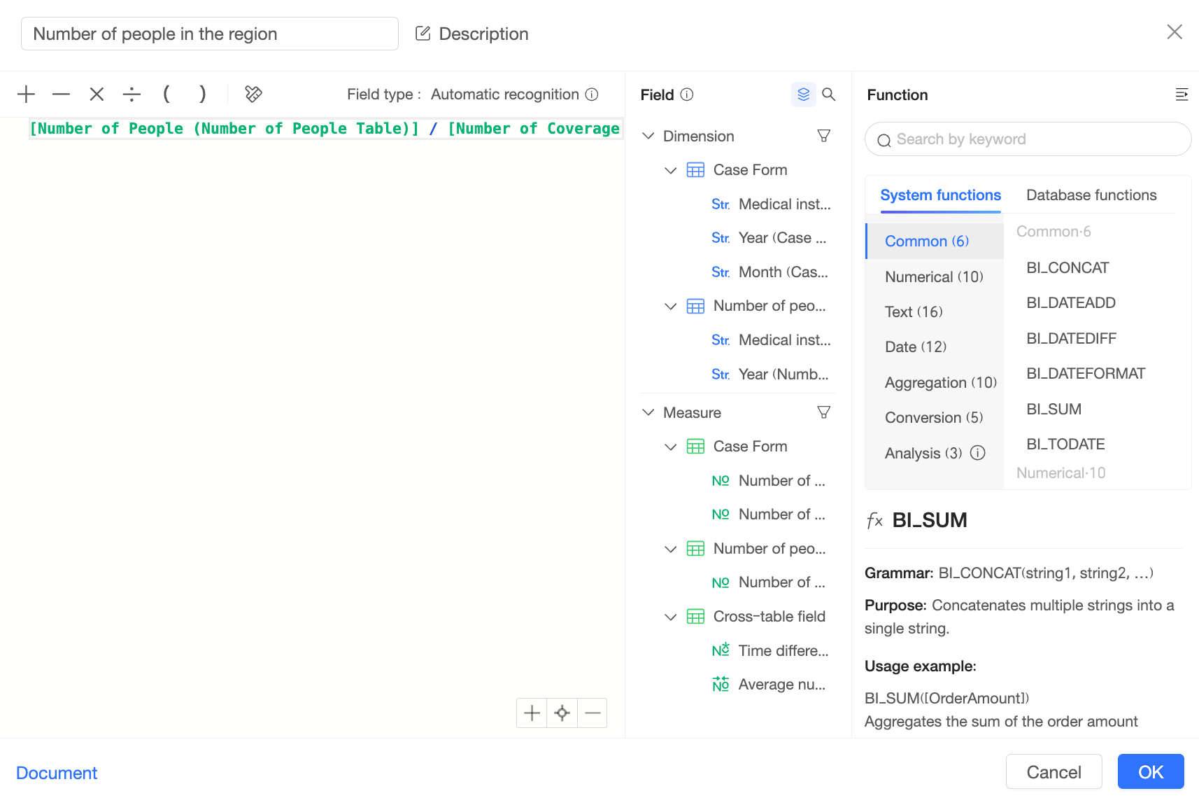
For example:
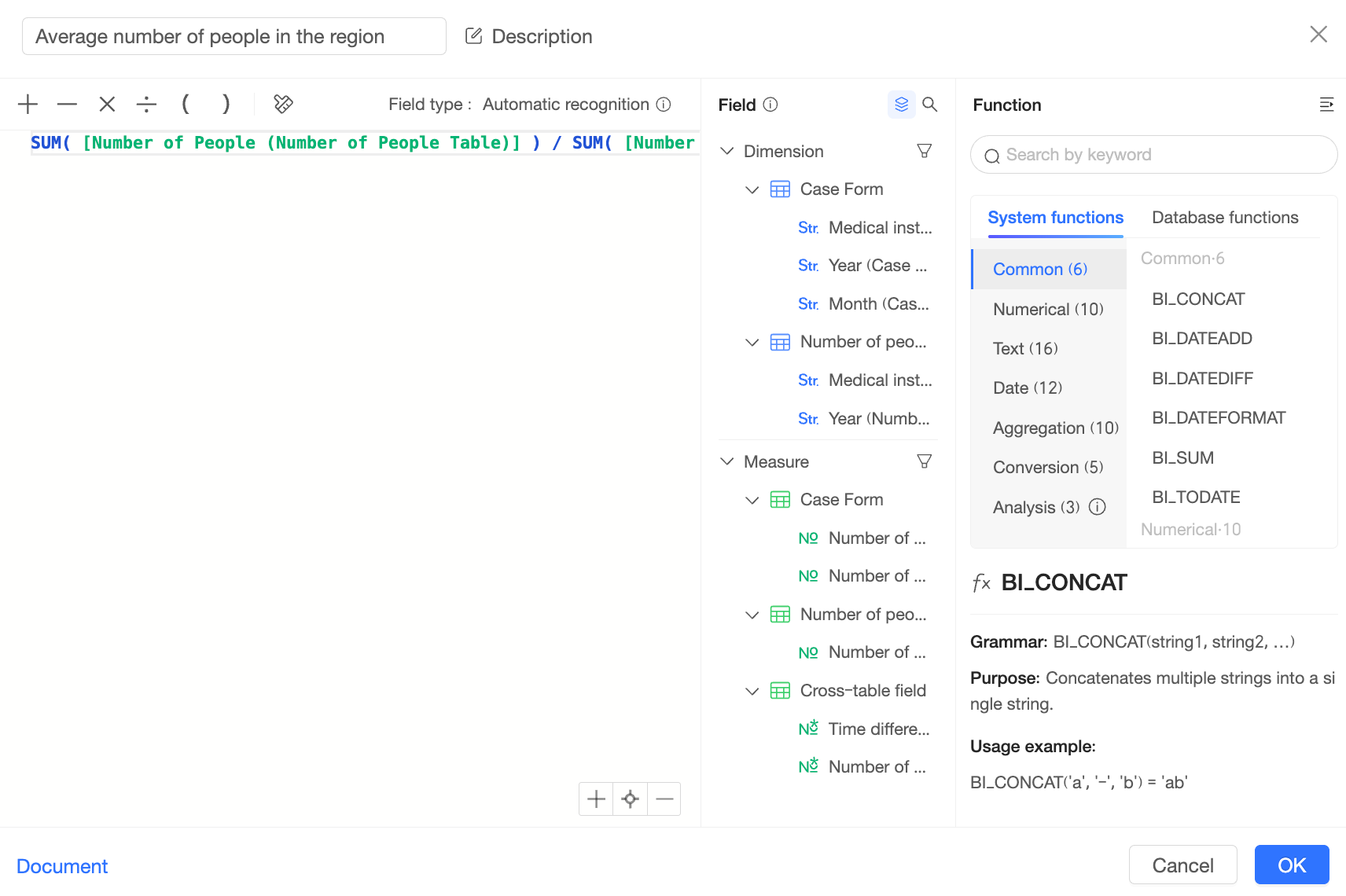
To compute this field, Quick BI first calculates SUM([Number of people(Table of Numbers)]) from the people count table and SUM([Coverage Area(Medical institution)]) from the case table, generating the following two intermediate tables:
|
Medical institution (case table) |
SUM(Number of people (people count table)) |
|
A |
210 |
|
B |
155 |
|
C |
160 |
|
- |
120 |
|
Medical institution (case table) |
SUM(Number of covered areas (case table)) |
|
A |
3 |
|
B |
2 |
|
C |
4 |
|
D |
1 |
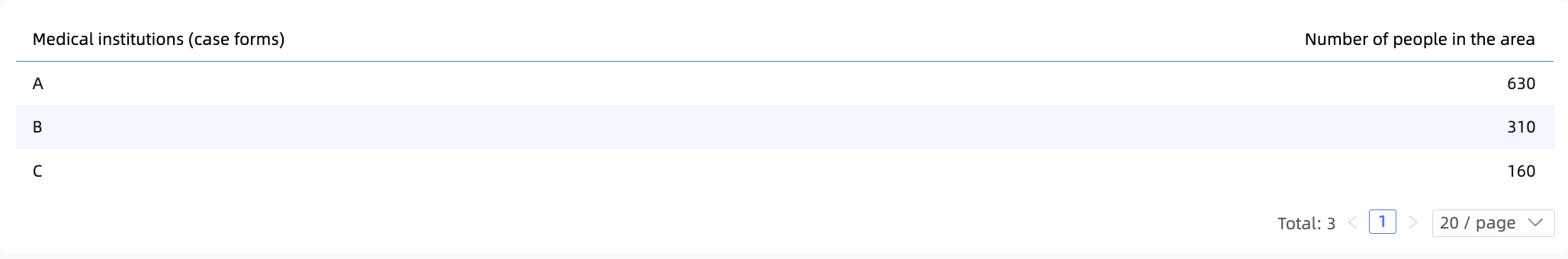
Quick BI then joins these two intermediate tables and performs the division to calculate the final result.
Detail-level cross-table fields
You create a detail-level cross-table field by using fields from single tables in a cross-table calculation at the detail level before any aggregation.
For example:
To compute this field, Quick BI first joins the "case table" and the "people count table" on their join keys to create the following intermediate table:
|
Medical institution (case table) |
Number of covered areas (case table) |
Medical institution (people count table) |
Number of people (people count table) |
|
A |
1 |
A |
110 |
|
A |
1 |
A |
100 |
|
B |
1 |
B |
75 |
|
B |
1 |
B |
80 |
|
C |
2 |
C |
90 |
|
C |
2 |
C |
70 |
|
A |
1 |
A |
110 |
|
A |
1 |
A |
100 |
|
B |
1 |
B |
75 |
|
B |
1 |
B |
80 |
|
C |
2 |
C |
90 |
|
C |
2 |
C |
70 |
|
A |
1 |
A |
110 |
|
A |
1 |
A |
100 |
Quick BI then performs the division on this intermediate table and aggregates the results based on the dimensions in the chart to produce the final result:
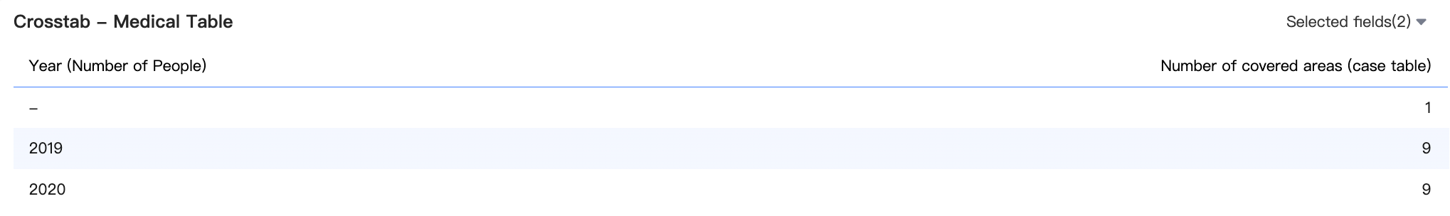
Handling constants
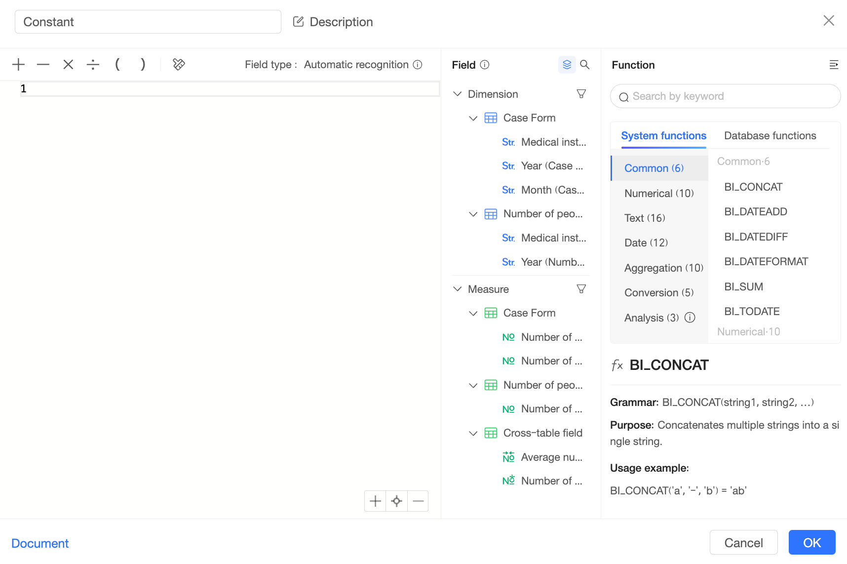
In a relational model, Quick BI treats constants (such as plain text or numeric literals) as cross-table fields but computes them differently from other cross-table fields.
For example, if you create a constant '1' in a relational model dataset, the field appears in the "Cross-Table Fields" category:
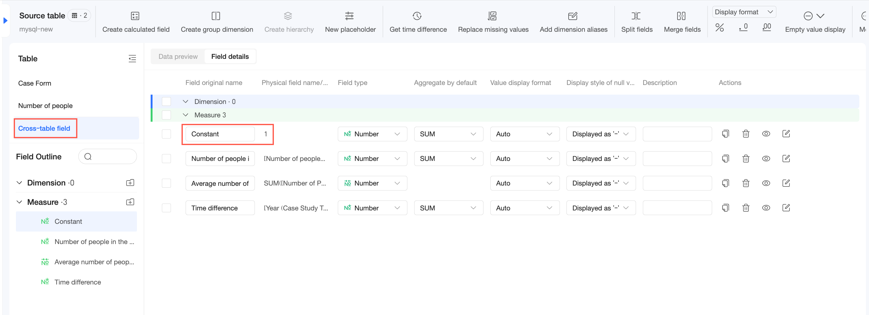
Constants in single-table calculations
In this case, Quick BI treats the constant as a field within that logical table. The calculation then follows the single-table query path, as shown below:
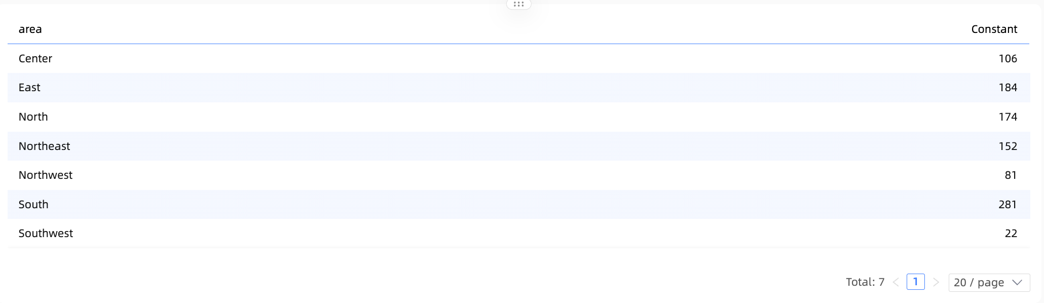
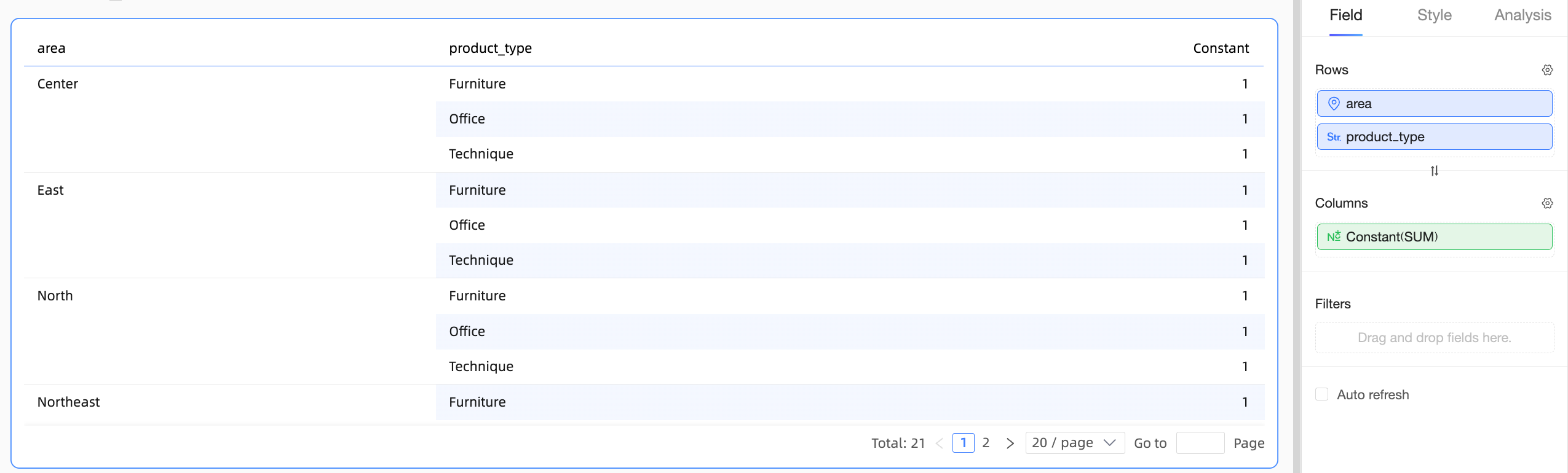
Constants in multi-table calculations
In this scenario, handling the constant becomes ambiguous. Associating the constant with different tables would produce different calculation results and could lead to unexpected outcomes.
In this scenario, Quick BI treats the constant as a cross-table field. The constant loses its association with dimensions in all tables and does not participate in aggregation. The effect is shown below: