Quick BI:Analytics Functions (LOD Functions)

Limits

Detail tables do not support LOD functions.

Background

Quick BI analysis currently relies on fixed dimensions. For example, to view order counts by region and province, place region and province (dimensions) on the rows of a cross table and order count (measure) on the columns. Set the aggregation method to Sum.

The generated SQL query is:

SELECT
  ADR_T_1_.`area` AS T_AAC_2_,
  ADR_T_1_.`province` AS T_A9E_3_,
  SUM(ADR_T_1_.`order_amt`) AS T_AAD_4_
FROM
  `qbi4test`.`company_sales_record` AS ADR_T_1_
GROUP BY
  ADR_T_1_.`area`,
  ADR_T_1_.`province`
ORDER BY
  T_AAC_2_ ASC,
  T_A9E_3_ ASC

But what if you want to see both region-province-level data and region-level data in the same table? Or compare province-level sales with region-level totals? Or identify the product type with the highest sales per province? In these cases, use LOD functions.

Scenarios

A Level of Detail expression defines the granularity level of data aggregation. Different levels represent different aggregation depths and granularities. LOD expressions handle visualizations that contain multiple detail levels.

If your analysis requires adding a dimension whose granularity is higher or lower than the current visualization—but you do not want to change the existing chart—use Level of Detail expressions.

Syntax

LOD (Level of Detail Expressions) is a powerful calculation feature. It enables complex calculations and aggregations during data analysis. LOD expressions control calculation granularity. They let you analyze data at a specified granularity level (FIXED), a higher granularity level (INCLUDE), or a lower granularity level (EXCLUDE). Basic usage follows:

LOD_FIXED

LOD_INCLUDE

LOD_EXCLUDE

Procedure

1. In the dataset editor, click Create Calculated Field to open the configuration dialog.

   

2. Enter a field name (①). In field expression, select the required LOD function and fields (②).

   

3. Click OK after creation. When you use the new field to build a dashboard chart, the total order amount for each region remains constant regardless of product type.

   

Expression Reference

Basic formula

The structure and syntax for the three LOD expressions are:

• Structure

  • LOD_FIXED{<dimension declaration> : <aggregation expression>}

  • LOD_INCLUDE{<dimension declaration> : <aggregation expression>}

  • LOD_EXCLUDE{<dimension declaration> : <aggregation expression>}

Example: LOD_FIXED{[order date]:sum([order amount])}

• Syntax reference

  • FIXED | INCLUDE | EXCLUDE: Keywords that define the LOD scope.

  • <dimension declaration>: One or more dimensions to link the aggregation expression to. Separate dimensions with commas.

  • <aggregation expression>: The calculation to perform. Defines the target dimension.

Filter Conditions

Quick BI supports filter conditions in addition to basic expressions. Separate dimension declarations, aggregation expressions, and filters with colons.

• LOD_FIXED{dimension1,dimension2...:aggregation expression:filter condition}

• LOD_INCLUDE{dimension1,dimension2...:aggregation expression:filter condition}

• LOD_EXCLUDE{dimension1,dimension2...:aggregation expression:filter condition}

Implementation Logic

In practice, LOD expressions generate aggregated data. To provide rich views, this data often merges with raw data or other aggregation levels. In SQL, subqueries and JOIN operations achieve this. This section explains the implementation logic for FIXED, INCLUDE, and EXCLUDE LOD expressions.

FIXED Level

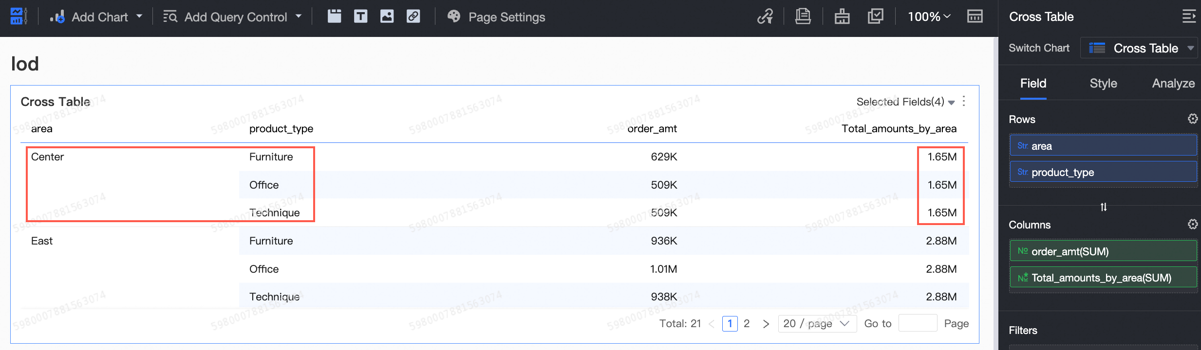
Recall the background question: How do you show both region-province-level data and region-level data in one table?

Create a FIXED expression:

LOD_FIXED{[area]:sum([order_amt])}

In SQL, use a subquery to calculate order totals per region, then JOIN it with the main query:

-- Simplified structure
-- lod_fixed{[area]:sum([order_amt])}
SELECT
    LOD_TM.`LOD_07AEF3F2F99A95` AS LOD_0,			-- area
    LOD_TM.`LOD_55512959145CF3` AS LOD_1,			-- province
    LOD_TM.`LOD_8BE7507A47AD81` AS LOD_2,			-- order_amt
    LOD_TP_0.`LOD_measure_result` AS LOD_3		-- lod_fixed{[area]:sum([order_amt])}
FROM
    (
        SELECT		-- Main query: area, province, sum(order_amt)
            ADR_T_1_.`area` AS LOD_07AEF3F2F99A95,
            ADR_T_1_.`province` AS LOD_55512959145CF3,
            SUM(ADR_T_1_.`order_amt`) AS LOD_8BE7507A47AD81
        FROM
            `qbi4test`.`company_sales_record` AS ADR_T_1_
        GROUP BY
            ADR_T_1_.`area`,
            ADR_T_1_.`province`
        ORDER BY
            LOD_07AEF3F2F99A95 ASC,
            LOD_55512959145CF3 ASC
        LIMIT
            0, 20
    ) AS LOD_TM
    INNER JOIN (
        SELECT			-- LOD subquery: area, sum(order_amt)
            ADR_T_1_.`area` AS LOD_07AEF3F2F99A95,
            sum(ADR_T_1_.`order_amt`) AS LOD_measure_result
        FROM
            `qbi4test`.`company_sales_record` AS ADR_T_1_
        GROUP BY
            ADR_T_1_.`area`
    ) AS LOD_TP_0 ON LOD_TM.`LOD_07AEF3F2F99A95` = LOD_TP_0.`LOD_07AEF3F2F99A95`


-- Standard structure
-- lod_fixed{[area]:sum([order_amt])}
SELECT
    LOD_TM.`LOD_07AEF3F2F99A95` AS LOD_0,
    LOD_TM.`LOD_55512959145CF3` AS LOD_1,
    LOD_TM.`LOD_8BE7507A47AD81` AS LOD_2,
    LOD_TP_0.`LOD_9D09E63F2E93FA` AS LOD_3
FROM
    (
        SELECT
            SUM(ADR_T_1_.`order_amt`) AS LOD_8BE7507A47AD81,
            ADR_T_1_.`province` AS LOD_55512959145CF3,
            ADR_T_1_.`area` AS LOD_07AEF3F2F99A95
        FROM
            `qbi4test`.`company_sales_record` AS ADR_T_1_
        GROUP BY
            ADR_T_1_.`province`,
            ADR_T_1_.`area`
        ORDER BY
            LOD_07AEF3F2F99A95 ASC,
            LOD_55512959145CF3 ASC
        LIMIT
            0, 20
    ) AS LOD_TM
    INNER JOIN (
        SELECT
            LOD_TL.`LOD_07AEF3F2F99A95` AS LOD_07AEF3F2F99A95,
            LOD_TL.`LOD_55512959145CF3` AS LOD_55512959145CF3,
            SUM(LOD_TR.`LOD_measure_result`) AS LOD_9D09E63F2E93FA
        FROM
            (
                SELECT
                    ADR_T_1_.`province` AS LOD_55512959145CF3,
                    ADR_T_1_.`area` AS LOD_07AEF3F2F99A95
                FROM
                    `qbi4test`.`company_sales_record` AS ADR_T_1_
                GROUP BY
                    ADR_T_1_.`province`,
                    ADR_T_1_.`area`
            ) AS LOD_TL
            INNER JOIN (
                SELECT
                    sum(ADR_T_1_.`order_amt`) AS LOD_measure_result,
                    ADR_T_1_.`area` AS LOD_07AEF3F2F99A95
                FROM
                    `qbi4test`.`company_sales_record` AS ADR_T_1_
                GROUP BY
                    ADR_T_1_.`area`
            ) AS LOD_TR ON LOD_TL.`LOD_07AEF3F2F99A95` = LOD_TR.`LOD_07AEF3F2F99A95`
        GROUP BY
            LOD_TL.`LOD_07AEF3F2F99A95`,
            LOD_TL.`LOD_55512959145CF3`
    ) AS LOD_TP_0 ON LOD_TM.`LOD_07AEF3F2F99A95` = LOD_TP_0.`LOD_07AEF3F2F99A95`
    AND LOD_TM.`LOD_55512959145CF3` = LOD_TP_0.`LOD_55512959145CF3`

INCLUDE Level

How do you show region-level data and the share of the top-selling province in each region?

Create an INCLUDE expression:

MAX(LOD_INCLUDE{[province]:SUM([order_amt])}) / SUM([order_amt])

In SQL, use a subquery to calculate order totals per region-province, then JOIN it with the main query:

-- Simplified structure
-- MAX(lod_include{[province]:SUM([order_amt])}) / SUM([order_amt])
SELECT
    LOD_TM.`LOD_07AEF3F2F99A95` AS LOD_0,		-- area
    LOD_TP_0.`LOD_EC796C51A8ABAB` / LOD_TM.`temp_calculation_0` AS LOD_1  -- MAX(lod_include{[province]:SUM([order_amt])}) / SUM([order_amt])
FROM
    (
        SELECT	-- Main query: area, sum(order_amt)
            ADR_T_1_.`area` AS LOD_07AEF3F2F99A95,
            sum(ADR_T_1_.`order_amt`) AS temp_calculation_0
        FROM
            `qbi4test`.`company_sales_record` AS ADR_T_1_
        GROUP BY
            ADR_T_1_.`area`
        ORDER BY
            LOD_07AEF3F2F99A95 ASC
        LIMIT
            0, 20
    ) AS LOD_TM
    INNER JOIN (		
        SELECT		-- LOD subquery: area, max(order_amt)
            LOD_TP_0.`LOD_07AEF3F2F99A95` AS LOD_07AEF3F2F99A95,
            MAX(LOD_TP_0.`LOD_measure_result`) AS LOD_EC796C51A8ABAB
        FROM
            (
                SELECT		-- area, province, sum(order_amt)
                    ADR_T_1_.`area` AS LOD_07AEF3F2F99A95,
                    ADR_T_1_.`province` AS LOD_55512959145CF3,
                    SUM(ADR_T_1_.`order_amt`) AS LOD_measure_result
                FROM
                    `qbi4test`.`company_sales_record` AS ADR_T_1_
                GROUP BY
                    ADR_T_1_.`area`,
                    ADR_T_1_.`province`
            ) AS LOD_TP_0 ON LOD_TM.`LOD_07AEF3F2F99A95` = LOD_TP_0.`LOD_07AEF3F2F99A95`

      
-- Standard structure
-- MAX(lod_include{[province]:SUM([order_amt])}) / SUM([order_amt])
SELECT
    LOD_TM.`LOD_07AEF3F2F99A95` AS LOD_0,
    LOD_TP_0.`LOD_EC796C51A8ABAB` / LOD_TM.`temp_calculation_0` AS LOD_1
FROM
    (
        SELECT
            ADR_T_1_.`area` AS LOD_07AEF3F2F99A95,
            sum(ADR_T_1_.`order_amt`) AS temp_calculation_0
        FROM
            `qbi4test`.`company_sales_record` AS ADR_T_1_
        GROUP BY
            ADR_T_1_.`area`
        ORDER BY
            LOD_07AEF3F2F99A95 ASC
        LIMIT
            0, 20
    ) AS LOD_TM
    INNER JOIN (
        SELECT
            LOD_TL.`LOD_07AEF3F2F99A95` AS LOD_07AEF3F2F99A95,
            MAX(LOD_TR.`LOD_measure_result`) AS LOD_EC796C51A8ABAB
        FROM
            (
                SELECT
                    ADR_T_1_.`province` AS LOD_55512959145CF3,
                    ADR_T_1_.`area` AS LOD_07AEF3F2F99A95
                FROM
                    `qbi4test`.`company_sales_record` AS ADR_T_1_
                GROUP BY
                    ADR_T_1_.`province`,
                    ADR_T_1_.`area`
            ) AS LOD_TL
            INNER JOIN (
                SELECT
                    SUM(ADR_T_1_.`order_amt`) AS LOD_measure_result,
                    ADR_T_1_.`province` AS LOD_55512959145CF3,
                    ADR_T_1_.`area` AS LOD_07AEF3F2F99A95
                FROM
                    `qbi4test`.`company_sales_record` AS ADR_T_1_
                GROUP BY
                    ADR_T_1_.`province`,
                    ADR_T_1_.`area`
            ) AS LOD_TR ON LOD_TL.`LOD_07AEF3F2F99A95` = LOD_TR.`LOD_07AEF3F2F99A95`
        GROUP BY
            LOD_TL.`LOD_07AEF3F2F99A95`
    ) AS LOD_TP_0 ON LOD_TM.`LOD_07AEF3F2F99A95` = LOD_TP_0.`LOD_07AEF3F2F99A95`

EXCLUDE Level

The FIXED LOD expression directly specifies a dimension like area to get region-level data. But what if you already added area and province to the chart? Can you exclude province and recalculate? Yes. That is the idea behind EXCLUDE LOD expressions.

Create an EXCLUDE expression:

LOD_EXCLUDE{[province]:SUM([order_number])}

In SQL, use a subquery to calculate order totals per region, then JOIN it with the main query:

-- Simplified structure
-- lod_EXCLUDE{[province]:SUM([order_number])}
SELECT
    LOD_TM.`LOD_07AEF3F2F99A95` AS LOD_0,       -- area
    LOD_TM.`LOD_55512959145CF3` AS LOD_1,       -- province
    LOD_TM.`LOD_140423A9870F07` AS LOD_2,       -- order_number
    LOD_TP_0.`LOD_measure_result` AS LOD_3      -- lod_EXCLUDE{[province]:SUM([order_number])}
FROM
    (
        SELECT      -- Main query: area, province, sum(order_number)
            ADR_T_1_.`area` AS LOD_07AEF3F2F99A95,
            ADR_T_1_.`province` AS LOD_55512959145CF3,
            SUM(ADR_T_1_.`order_number`) AS LOD_140423A9870F07
        FROM
            `qbi4test`.`company_sales_record` AS ADR_T_1_
        GROUP BY
            ADR_T_1_.`area`,
            ADR_T_1_.`province`
        ORDER BY
            LOD_07AEF3F2F99A95 ASC,
            LOD_55512959145CF3 ASC
        LIMIT
            0, 20
    ) AS LOD_TM
    INNER JOIN (
        SELECT      -- LOD subquery: area, sum(order_number)
            ADR_T_1_.`area` AS LOD_07AEF3F2F99A95,
            SUM(ADR_T_1_.`order_number`) AS LOD_measure_result
        FROM
            `qbi4test`.`company_sales_record` AS ADR_T_1_
        GROUP BY
            ADR_T_1_.`area`
    ) AS LOD_TP_0 ON LOD_TM.`LOD_07AEF3F2F99A95` = LOD_TP_0.`LOD_07AEF3F2F99A95`
    AND LOD_TM.`LOD_55512959145CF3` = LOD_TP_0.`LOD_55512959145CF3`



-- Standard structure
-- lod_EXCLUDE{[province]:SUM([order_number])}
SELECT
    LOD_TM.`LOD_07AEF3F2F99A95` AS LOD_0,
    LOD_TM.`LOD_55512959145CF3` AS LOD_1,
    LOD_TM.`LOD_140423A9870F07` AS LOD_2,
    LOD_TP_0.`LOD_90EDFE3F5B628A` AS LOD_3
FROM
    (
        SELECT
            SUM(ADR_T_1_.`order_number`) AS LOD_140423A9870F07,
            ADR_T_1_.`province` AS LOD_55512959145CF3,
            ADR_T_1_.`area` AS LOD_07AEF3F2F99A95
        FROM
            `qbi4test`.`company_sales_record` AS ADR_T_1_
        GROUP BY
            ADR_T_1_.`province`,
            ADR_T_1_.`area`
        ORDER BY
            LOD_07AEF3F2F99A95 ASC,
            LOD_55512959145CF3 ASC
        LIMIT
            0, 20
    ) AS LOD_TM
    INNER JOIN (
        SELECT
            LOD_TL.`LOD_07AEF3F2F99A95` AS LOD_07AEF3F2F99A95,
            LOD_TL.`LOD_55512959145CF3` AS LOD_55512959145CF3,
            SUM(LOD_TR.`LOD_measure_result`) AS LOD_90EDFE3F5B628A
        FROM
            (
                SELECT
                    ADR_T_1_.`province` AS LOD_55512959145CF3,
                    ADR_T_1_.`area` AS LOD_07AEF3F2F99A95
                FROM
                    `qbi4test`.`company_sales_record` AS ADR_T_1_
                GROUP BY
                    ADR_T_1_.`province`,
                    ADR_T_1_.`area`
            ) AS LOD_TL
            INNER JOIN (
                SELECT
                    SUM(ADR_T_1_.`order_number`) AS LOD_measure_result,
                    ADR_T_1_.`area` AS LOD_07AEF3F2F99A95
                FROM
                    `qbi4test`.`company_sales_record` AS ADR_T_1_
                GROUP BY
                    ADR_T_1_.`area`
            ) AS LOD_TR ON LOD_TL.`LOD_07AEF3F2F99A95` = LOD_TR.`LOD_07AEF3F2F99A95`
        GROUP BY
            LOD_TL.`LOD_07AEF3F2F99A95`,
            LOD_TL.`LOD_55512959145CF3`
    ) AS LOD_TP_0 ON LOD_TM.`LOD_07AEF3F2F99A95` = LOD_TP_0.`LOD_07AEF3F2F99A95`
    AND LOD_TM.`LOD_55512959145CF3` = LOD_TP_0.`LOD_55512959145CF3`

FIXED Function Examples

A FIXED Level of Detail expression calculates using only the specified dimensions. It ignores all others.

Example 1: Total sales amount per region

Scenario

You analyze regional sales orders. Your dataset includes region and province dimensions. Use FIXED to compute the total sales amount per region. FIXED ignores all other dimensions. So it returns the correct regional sales total.

Procedure

1. Create a calculated field.

   Field expression: LOD_FIXED{[region]:BI_SUM([order amount])}

   Meaning: Sum order amount by region.

   

2. Create a chart.

   This example uses a cross table.

   Drag the Regional Amount Sum field into the column area. Drag region and province into the row area. Click Update. The system updates the chart automatically.

   

   Now, the regional amount sum stays constant across provinces.

Example 2: Customer order frequency

Scenario description

A sales manager wants to know how many customers placed one, two, or three orders—and so on. Analyze customer repeat purchase behavior by counting order frequency per customer. Use a Level of Detail expression to group one measure by another.

This example uses LOD_FIXED to convert order count into a customer-count dimension. Compute customer order frequency.

Procedure

1. Create a calculated field.

   Field expression: LOD_FIXED{[customer name]:COUNT([order id])}

   Meaning: Count purchase frequency per customer.

2. Create a chart.

   This example uses a column chart.

   Drag the Purchase Frequency field into the category axis/dimension area. Drag customer name into the axis value/measure area and set it to distinct count. Click Update. The system updates the chart automatically.

   

Now, you see that the most common purchase frequency is seven. One customer ordered 58 times.

Example 3: Regional profit percentage ranking

Scenario

A regional sales director wants to know each region’s share of total profit—and quickly identify top contributors. You can use Advanced Calculation → Percentage. Or use Level of Detail expressions for more flexibility.

This example uses LOD_FIXED to compute regional profit percentage ranking.

Procedure

1. Create a calculated field.

   1. Field expression: LOD_FIXED{:SUM([profit amount])}

      Meaning: This FIXED expression omits dimensions. So it sums profit without grouping.

   2. Divide SUM([profit amount]) by the LOD result: SUM([profit amount]) / SUM(LOD_FIXED{:SUM([profit amount])}). This gives each region’s profit share.

      

2. Create a chart.

   In this example, you create a leaderboard.

   Drag the Profit Share Percentage field into the metric/measure area. Drag area into the category/dimension area. Click Update. The system updates the chart automatically.

   

Now, South China and North China rank highest. East China and Southwest rank lowest—and even show negative profit. East China data looks like dirty data.

Example 4: Annual new user count

Scenario description

How do you know if your product grows positively? Beyond PV and UV, track customer loyalty. Users who stay long and keep ordering show strong product stickiness. Use Level of Detail expressions to measure this.

This example uses LOD_FIXED to compute annual new user count.

Procedure

1. Create a calculated field.

   Field expression: LOD_FIXED{[customer name]:MIN(DATE_FORMAT([buy date], '%Y'))}

   Meaning: Find each user’s earliest order year. Adjust granularity as needed using database-compatible date functions.

2. Create a chart.

   This example uses a line chart.

   Drag the Customer First Purchase Year field into the category axis/dimension area. Drag sales amount into the axis value/measure area. Click Update. The system updates the chart automatically.

   

Now, users who started in 2013 still contribute heavily. Product stickiness remains high.

Example 5: New customer count trend by year from order details

Scenario

Count unique customers per first-purchase year. Then analyze distribution.

Procedure

1. Create calculated fields.

   1. Field 1: LOD_FIXED{[customer ID]: min(BI_YEAR([order date]))}

      Name this field Customer First Purchase Year. Set data type to dimension and field type to text.

   2. Field 2: Customer Count=count(distinct [customer ID])

2. Create a chart.

   This example uses a column chart. Drag Customer First Purchase Year into the category axis/dimension area. Drag Customer Count into the value axis/measure area. Click Update. The system updates the chart automatically.

   

Now, you see annual new customer counts. 2021 had the most. Counts dropped sharply afterward.

Example 6: Customer count distribution by purchase frequency from order details

Scenario

Count purchases per customer. Then analyze distribution.

Procedure

1. Create calculated fields.

   1. Field 1: LOD_FIXED{[customer ID]: count(distinct [order ID])}

      Name this field Customer Purchase Frequency. Set data type to dimension and field type to text.

   2. Field 2: Customer Count=count(distinct [customer ID])

2. Create a chart.

   This example uses a column chart. Drag Customer Purchase Frequency into the category axis/dimension area. Drag Customer Count into the value axis/measure area. Click Update. The system updates the chart automatically.

   

In this case, the customer count is highest for a purchase frequency of 3.

Example 7: Compare yearly order amounts with key year 2023

Scenario

Compare yearly order data against a key year—2023.

Procedure

1. Create a calculated field.

   sum([order amount])/
   LOD_FIXED{:
   sum(
   case when BI_YEAR([order date]) ='2023' 
   then [order amount] else 
   0 end)} 
   -1

   Breakdown:

   1. Calculate 2023 order amount: LOD_FIXED{:sum(case when BI_YEAR([order date]) ='2023' then [order amount] else 0 end)}

   2. Compare yearly order amounts with 2023 order amount: sum([order amount])/[2023 order amount]-1. Name this field vs. 2023.

2. Create a chart.

   This example uses a cross table. Drag order date (year) into the row area. Drag order amount and vs. 2023 into the column area. Click Update. The system updates the chart automatically.

   

Now, you see yearly order amounts and comparisons with 2023.

Example 8: Profit and loss day count analysis by year and month

Scenario

Tag each day as profitable or unprofitable based on daily profit. Then count days by tag, year, and month.

Procedure

1. Create calculated fields.

   1. Field 1:

      case when 
      LOD_FIXED{[order date]:sum([profit])}>0 
      then 'Profitable' 
      else 'Unprofitable' 
      end

      Name this field Day Profit/Loss Tag. Set data type to dimension and field type to text.

      Breakdown:

      1. Sum profit by order date: LOD_FIXED{[order date]:sum([profit])}

      2. If profit sum > 0, return “Profitable”. Else return “Unprofitable”: case when [profit sum]>0 then 'Profitable' else 'Unprofitable' end

   2. Field 2: Days=count(distinct [order date])

   3. Field 3: Month=BI_MONTH([order date])

2. Create charts.

   Use split dimensions in line-column charts to make small multiples. Visualize trends as stacked or categorical. See clear comparisons and patterns.

   This example creates a stacked column chart for profit/loss day distribution (stacked trend). It also creates two area charts for profit/loss day distribution.

   1. Create a stacked column chart. Drag Month into the category axis/dimension area. Drag Days into the value axis/measure area. Drag Day Profit/Loss Tag into the color legend/dimension area. Drag order date (year) into the split/dimension area. Click Update. The system updates the chart automatically.

      

   2. Create two area charts—one for unprofitable days, one for profitable days.

      In both charts, drag Month into the category axis/dimension area. Drag Days into the value axis/measure area. Drag order date (year) into the split/dimension area.

      Add Day Profit/Loss Tag to the filter. Set exact match to “Unprofitable” for the first chart. Set exact match to “Profitable” for the second.

      

      Click Update. The system updates the charts automatically.

      

Now, you see clear comparisons and trends for profit/loss days by year and month.

INCLUDE Function Examples

An INCLUDE Level of Detail expression groups calculations by the specified dimensions. INCLUDE adds one more layer of analysis on top of existing granularity.

Example 1: Average customer sales amount

Scenario

When analyzing product sales, you need average customer sales amount. Use INCLUDE to compute each customer’s total order amount. Then use average aggregation.

Procedure

1. Create a calculated field.

   Field expression: LOD_INCLUDE{[user id]:SUM([order amount])}

   Meaning: Sum order amount per user ID.

   

2. Create a chart.

   This example uses a cross table.

   Drag order amount and Customer Order Total into the column area. Drag product type into the row area. Set Customer Order Total aggregation to Average. Click Update. The system updates the chart automatically.

Now, you see average customer sales amount per product type.

Example 2: Average maximum transaction amount per sales representative

Scenario

A sales director needs the average of each sales representative’s largest transaction, grouped by region—and shown on a map. Use Level of Detail expressions to display data at the region level. Drill down to sales representatives to see which regions perform well or poorly. Then plan goals accordingly.

This example uses LOD_INCLUDE to compute average maximum transaction amount per sales representative.

Procedure

1. Create a calculated field.

   Field expression: AVG(LOD_INCLUDE{[sales name]:MAX([price])})

   Meaning: Add sales representative name as an analysis dimension. Then compute the average of maximum transaction amounts.

   

2. Create a chart.

   This example uses a colored map.

   1. Drag Average Maximum Sales Amount per Region into the color saturation/measure area. Drag area into the geographic region axis/dimension area.

   2. In Style → Blocks, highlight the region with the maximum value in red.

      

      Click Update. The system updates the chart automatically.

      

Now, East China shows higher maximum sales. Northwest and Southwest show lower values.

Example 3: Total profit for regions where order amount exceeds 500,000

Scenario description

Sum order amounts by region. Then compute total profit for regions where order amount exceeds 500,000.

Procedure

1. Create a calculated field.

   CASE WHEN LOD_INCLUDE{[region]:BI_SUM([order amount])}>500000 
   then [profit amount] 
   else 0 
   end

   Breakdown:

   1. Compute order amount per region. Name this field Region Order Amount: LOD_INCLUDE{[region]:BI_SUM([order amount])}

   2. Find regions where order amount exceeds 500,000 and sum their profit: CASE WHEN [Region Order Amount]>500000 then [profit amount] else 0 end

   3. Sum results (using SUM or setting chart field aggregation to Sum) to get total profit for qualifying regions.

2. Create charts.

   This example uses a scorecard to display data. You can also create a cross table to verify accuracy. In the scorecard, drag the new field into the scorecard metric/measure area. Set field aggregation to Sum. In the cross table, drag region into the row area. Drag order amount, profit amount, and the new field into the column area. Set field aggregation to Sum. Click Update. The system updates the charts automatically.

   

   Now, Northeast, East China, North China, and South China exceed 500,000 in order amount. Their total profit is 459,000 CNY.

Example 4: Total profit for regions where train-shipped order amount exceeds 100,000 per product type

Scenario

This is an upgrade of Example 3. It adds train shipping and product type grouping. Compute total profit for regions where train-shipped order amount exceeds 100,000 per product type. This involves nested functions. Break them down for clarity.

Procedure

1. Create a calculated field:

   SUM(
   CASE WHEN LOD_INCLUDE{[product type],[region]:sum(if([shipping method]='train',[order amount],0))}>100000
   then [profit amount]
   else 0
   end)

   Breakdown:

   1. Sum train-shipped order amounts per product type and region. Name this field Product Type–Region Order Amount: LOD_INCLUDE{[product type],[region]:sum(if([shipping method]='train',[order amount],0))}

   2. Find regions where order amount exceeds 100,000 and sum their profit: CASE WHEN [Product Type–Region Order Amount]>100000 then [profit amount] else 0 end

   3. Sum results.

2. Create charts.

   1. Create two scorecards. In Scorecard 1, drag the new field into the scorecard metric/measure area. In Scorecard 2, drag the new field into the scorecard metric/measure area and drag product type into the scorecard tag/dimension area. Click Update. The system updates the charts automatically.

      

      Now, total profit for train-shipped orders over 100,000 is 426,000 CNY. Office supplies: 147,200 CNY. Furniture: 0 CNY. Technology: 278,800 CNY.

   2. Create a cross table to verify accuracy. Drag product type, shipping method, and region into the row area. Drag order amount, profit amount, and the new field into the column area. Click Update. The system updates the chart automatically.

      For office supplies, train-shipped orders over 100,000 occur in Northeast, East China, North China, and South China. Their total profit is 147,200 CNY—matching the scorecard. Verify other product types similarly.

Example 5: Customer count for regions where train-shipped order amount exceeds 100,000 per product type

Scenario

This resembles Example 4, but computes customer count instead of profit.

Procedure

1. Create a calculated field:

   COUNT(DISTINCT(
   CASE WHEN LOD_INCLUDE{[product type],[region]:sum(if([shipping method]='train',[order amount],0))}>100000
   then [user id]
   else null
   end))

   Breakdown:

   1. Sum train-shipped order amounts per product type and region. Name this field Product Type–Region Order Amount: LOD_INCLUDE{[product type],[region]:sum(if([shipping method]='train',[order amount],0))}

   2. Find regions where order amount exceeds 100,000 and list their customers: CASE WHEN [Product Type–Region Order Amount]>100000 then [user id] else null end

   3. Finally, use COUNT(DISTINCT()) to count unique values.

2. Create a chart.

   This example uses a scorecard. Drag the new field into the scorecard metric/measure area. Click Update. The system updates the chart automatically.Now, customer count for train-shipped orders over 100,000 is 1,026.

Example 6: Count of regions where order amount exceeds 500,000

Scenario

This resembles Example 3, but counts regions instead of computing profit.

Procedure

1. Create a calculated field:

   COUNT(DISTINCT(
   CASE WHEN LOD_INCLUDE{[region]:sum([order amount])}>500000
   then [region]
   else null
   end))

   Breakdown:

   1. Compute order amount per region. Name this field Region Order Amount: LOD_INCLUDE{[region]:sum([order amount])}

   2. Find regions where order amount exceeds 500,000: CASE WHEN [Region Order Amount]>500000 then [region] else null end

   3. Finally, you can use COUNT(DISTINCT()) to count the unique items.

2. Create charts.

   This example uses a scorecard. You can also create a cross table to verify accuracy. In the scorecard, drag the new field into the scorecard metric/measure area. In the cross table, drag region into the row area and order amount into the column area. Click Update. The system updates the charts automatically.

   

   Now, four regions exceed 500,000 in order amount: Northeast, East China, North China, and South China.

Example 7: Average provincial sales amount per product type in 2024

Scenario

Compute average provincial sales amount per product type in 2024.

Procedure

1. Create a calculated field.

   AVG(
   LOD_INCLUDE{[product type],[province]:
   SUM(IF(YEAR([order date])='2024',[order amount],0))
   }
   )

   Breakdown:

   1. Compute order amount for 2024 orders. Name this field 2024 Order Amount: IF(YEAR([order date])='2024',[order amount],0)

   2. Sum sales by product type and province: LOD_INCLUDE{[product type],[province],SUM[2024 Order Amount]}

   3. Compute average.

2. Create charts.

   This example uses a scorecard. You can also create a cross table to verify accuracy. In the scorecard, drag the new field into the scorecard metric/measure area and drag product type into the scorecard tag/dimension area. In the cross table, drag product type into the row area and order amount into the column area. Filter for 2024 data. Click Update. The system updates the charts automatically.

   

   Now, office supplies’ 2024 order amount is 235,600 CNY. Average provincial sales is 235,600 ÷ 31 provinces = 7,600 CNY. Other product types follow the same logic.

Example 8: Average provincial customer count per product type in 2024

Scenario

This resembles Example 7, but computes average customer count instead of average sales.

Procedure

1. Create a calculated field.

   AVG(
   LOD_INCLUDE{[product type],[province]:
   COUNT(DISTINCT(IF(YEAR([order date])='2024',[user id],null)))
   }
   )

   Breakdown:

   1. Count customers for 2024 orders. Name this field 2024 Customer Count: IF(YEAR([order date])='2024',[user id],null)

   2. Count customers by product type and province: LOD_INCLUDE{[product type],[province],SUM[2024 Customer Count]}

   3. Compute average.

2. Create charts.

   This example uses a scorecard. You can also create a cross table to verify accuracy. In the scorecard, drag the new field into the scorecard metric/measure area and drag product type into the scorecard tag/dimension area. In the cross table, drag product type into the row area and Product Type Provincial Customer Count into the column area. Filter for 2024 data. Click Update. The system updates the charts automatically.

   Product Type Provincial Customer Count=LOD_INCLUDE{[product type],[province]:COUNT(DISTINCT([user id]))}

   

   Now, office supplies’ 2024 provincial customer count is 212. Average provincial customer count is 212 ÷ 31 provinces = 6.839. Other product types follow the same logic.

Example 9: Product target achievement ratio and profit gap per province

Scenario

With known provincial profit targets, analyze which products meet or miss targets.

Compute profit gaps per product at the province level. Count products that meet targets. Count total products. Compute the ratio.

This scenario requires two linked charts. Click left-side product stats to view right-side product details.

Procedure

1. Create calculated fields.

   1. Field 1: Product Profit Target Gap

      LOD_INCLUDE{[product] : sum([profit]-[profit target])}.

      Meaning: Compute profit target gap per product.

   2. Field 2: Target Achievement Ratio

      count(distinct 
      case when [Product Profit Target Gap]>0 
      then [product] 
      else null end)
      /count(distinct [product])

      Breakdown:

      1. Count distinct products where profit target gap > 0. Name this Products That Meet Targets: count(distinct case when [Product Profit Target Gap]>0 then [product] else null end)

      2. Count distinct total products: count(distinct [product])

      3. Divide the two: [Products That Meet Targets]/[Total Products]. This gives Target Achievement Ratio.

2. Create charts.

   This example creates two charts with interaction.

   1. Create a bar chart for Product Profit Target Gap. Drag product into the category axis/dimension area. Drag Product Profit Target Gap into the value axis/measure area. Click Update. The system updates the chart automatically.

      

   2. Create a bar chart for Target Achievement Ratio. Drag province into the category axis/dimension area. Drag Target Achievement Ratio into the value axis/measure area. Click Update. The system updates the chart automatically.

      

   3. Configure interaction between the two bar charts.

      Note

      In this example, both charts use the same dataset. If auto-interaction is enabled, charts link automatically. If disabled, configure manual interaction.

      For details, see Interaction.

      Interaction preview.

Now, you see provincial profit target progress and which products meet or miss targets.

Example 10: Store performance evaluation by region

Scenario

Using store-level sales and gross profit data, compute total sales and gross profit per region. Also compute average sales and gross profit per store. Use filters to view performance at regional or sub-regional levels.

Procedure

1. Create calculated fields.

   1. Field 1: Store Gross Profit=LOD_INCLUDE{[store name]:sum([gross profit])}

   2. Field 2: Store Sales Amount=LOD_INCLUDE{[store name]:sum([sales amount])}

2. Create a chart.

   This example uses a cross table with conditional formatting.

   1. In the cross table, drag Parent Region and Sub-region into the row area. In the column area, add two Store Gross Profit fields—one set to Average, one to Sum. Add two Store Sales Amount fields—one set to Average, one to Sum.

      

   2. Label Store Gross Profit (Average) and Store Sales Amount (Average) as Per Store. Label Store Gross Profit (Sum) and Store Sales Amount (Sum) as Total.

   3. In Style → Cell → Metric Grouping, set Metric Grouping.

      

   4. Apply conditional formatting for aesthetics. This example configures all four columns as follows:

   5. Click Update. The system updates the chart automatically.

Now, you see total and per-store sales and gross profit for each region.

Example 11: Regional evaluation based on provincial performance

Scenario

By province, compute sales per region. Count provinces where sales exceed a threshold (set via filter). Also compute total customers in those provinces and average customers per province. Change the threshold to see updated results.

Procedure

1. Create calculated fields.

   1. Field 1: Qualified Province Count

      count(distinct 
      case when LOD_INCLUDE{[province]:sum([order amount])} > $val{ord_amt_level} 
      then [province] 
      else null
      end)

      Breakdown:

      1. Compute order amount per province: LOD_INCLUDE{[province]:sum([order amount])}. Name this Province Order Amount.

      2. Return province if Province Order Amount > value placeholder ord_amt_level. Else return null: case when [Province Order Amount]> $val{ord_amt_level} then [province] else null end. Name this Qualified Provinces.

      3. Count distinct qualified provinces: count(distinct [Qualified Provinces]).

   2. Field 2: Total Customers in Qualified Provinces

      count(distinct 
      case when lod_include{[province]:sum([order amount])} > $val{ord_amt_level} 
      then [customer ID] 
      else null 
      end)

      Breakdown:

      1. Compute order amount per province: LOD_INCLUDE{[province]:sum([order amount])}. Name this Province Order Amount.

      2. Return customer ID if Province Order Amount > value placeholder ord_amt_level. Else return null: case when [Province Order Amount]> $val{ord_amt_level} then [customer ID] else null end. Name this Customers in Qualified Provinces.

      3. Count distinct Customers under Province. Formula: count(distinct [Customers under Province])

   3. Field 3: Average Customers Per Province = [Total Customers in Qualified Provinces] ÷ [Qualified Province Count].

2. Create charts.

   1. Create a cross table. Drag region into the row area. Drag Province Count, Province Customer Count, and Average Customers Per Province into the column area.

   2. Add an internal query filter. Set filter to province sales amount. Link to value placeholder ord_amt_level. Set default value to 100000.

   3. Click Update. The system updates the chart automatically.

      

Now, change the province sales amount to see updated results.

EXCLUDE Function Examples

An EXCLUDE Level of Detail expression calculates after removing the specified dimensions.

Example 1: Province sales share within region

Scenario

When analyzing province-level sales within a region, you also need the region’s total sales and each province’s sales share. Use EXCLUDE to compute regional sales excluding the current province. Then sum to get the region’s total.

Procedure

1. Create a calculated field.

   Field expression: LOD_EXCLUDE{[province]:SUM([order amount])}

   Meaning: Compute regional sales excluding the current province.

   

2. Create a chart.

   This example uses a cross table. Drag order amount and Regional Total Sales into the column area. Drag region and province into the row area. Click Update. The system updates the chart automatically.

   

Now, you see both province-level order amounts and regional total sales.

Example 2: Difference between sales area and battle zone averages

Scenario

A sales company has seven national battle zones. Each battle zone contains multiple sales areas by province. At year-end, quickly compare each province’s average sales profit against its battle zone’s overall average. Identify top-performing and underperforming zones. Use Level of Detail expressions and conditional formatting to build this report.

This example uses LOD_EXCLUDE to compute difference between sales area and battle zone averages.

Procedure

1. Create a calculated field.

   1. Field expression: AVG(LOD_EXCLUDE{[province]:AVG([price])})

      Meaning: Starting from the original setup, exclude sales regions from the aggregation granularity and compute the average sales across the remaining granularities. This expression calculates the average sales for each region, such as East China.

   2. Subtract the LOD result from AVG([price]): AVG([price]) - AVG(LOD_EXCLUDE{[province]:AVG([price])}). This gives the difference between each sales area and its battle zone average.

      

2. Create a chart.

   This example uses a cross table.

   1. Drag the Province Average Difference field into the column area. Drag area and province into the row area.

   2. In Style → Conditional Formatting, set this field to red if > 0 and green if < 0.

      

   3. Click Update. The system updates the chart automatically.

      

Now, Shanghai, Anhui, Jiangsu, and Fujian outperform the East China average. Shanghai leads. Shandong, Jiangxi, and Zhejiang fall short and need improvement.

Filter Condition Rules

LOD_FIXED + External Filters

• Results Unaffected by Filters

  LOD_FIXED_1 field expression: LOD_FIXED{[region]: SUM([order amount])}

  Filter: shipping method = “truck”

  Result explanation: As shown below, Northeast region’s total order amount is 527,400 CNY. With no external filter—or with shipping method = “truck”—Northeast’s total stays 527,400 CNY. Filters do not affect results.

  Conclusion: Filters unrelated to LOD aggregation dimensions do not affect results.

  

• Results Affected by Filters

  LOD_FIXED_2 field expression: LOD_FIXED{[region], [product type], [shipping method]: SUM([order amount])}

  Filter: shipping method = “truck”

  Result explanation: As shown below, Northeast–office supplies total is 150,800 CNY—sum of truck (35,540 CNY), train (103,100 CNY), and air (12,110 CNY). With shipping method = “truck”, Northeast–office supplies becomes 35,540 CNY—the amount for Northeast–office supplies–truck.

  Conclusion: Filters matching LOD aggregation dimensions affect results due to secondary aggregation.

  

LOD + Internal Filters

Conclusion: Internal filters matching LOD granularity apply to all related data. Otherwise, they apply only to the LOD field.

• LOD_FIXED

  • LOD_FIXED_3 field expression: LOD_FIXED{[region], [product type], [shipping method]: SUM([order amount]): [order level]='intermediate'}

    Calculation result: As shown in the following figure, the order amount for Northeast region → Office supplies → Large card is 35,070. This amount represents data filtered for orders with an Intermediate order level—that is, the order amount for Northeast region → Office supplies → Large card → Intermediate.

    

  • LOD_FIXED_4 field expression: LOD_FIXED{[region], [product type], [shipping method]: SUM([order amount]): [shipping method]='truck'}

    Result: As shown below, Northeast–office supplies–truck order amount is 355,400 CNY. When internal filters match LOD granularity, LOD_FIXED filters for truck shipments.

    

• LOD_INCLUDE

  LOD_EXCLUDE and LOD_INCLUDE follow the same logic. This example uses LOD_INCLUDE.

  

  • LOD_INCLUDE_1 field expression: LOD_INCLUDE{: SUM([order amount]): [order level]='intermediate'}

    Calculation result: As shown in the figure below, taking the Northeast region as an example, the order amount for 'Northeast Region-Office Supplies-Large Card' is 35,070. This amount is obtained by filtering for orders with a 'Medium' level, specifically representing 'Northeast Region-Office Supplies-Large Card-Medium'.

  • LOD_INCLUDE_2 field expression: LOD_INCLUDE{: SUM([order amount]): [shipping method]='truck'}

    Result: As shown below, Northeast–office supplies–truck order amount is 355,400 CNY. When internal filters match LOD granularity, LOD_INCLUDE filters for truck shipments.