PolarDB:High-dimensional vector search (PASE)

Background information

In recent years, representation learning, a key deep learning technology, has made significant progress. It is widely used in industries for applications such as ad delivery, facial recognition payments, image recognition, and speech recognition. Data is embedded into high-dimensional vectors, and vector search technology is then used to find related items.

The PostgreSQL ANN search extension (PASE) is a high-performance vector search index extension developed for PostgreSQL databases. It uses mature, stable, and efficient approximate nearest neighbor (ANN) search algorithms, including IVFFlat and HNSW. These algorithms enable extremely fast vector queries in PostgreSQL databases. PASE does not currently support feature vector extraction and generation. You must retrieve the feature vectors of entities yourself. PASE searches for similar vectors from large volumes of existing vectors.

Target audience

This topic does not provide detailed explanations of machine learning terms. To understand this topic, you need a basic knowledge of machine learning, search, and recommendation.

Precautions

• Indexes can become bloated. You can check the bloat rate by running the select pg_relation_size('index_name'); command. If the index size is much larger than the data size and queries slow down significantly, you must reindex.

• Indexes can become inaccurate after frequent data updates. If you require absolute accuracy, you should reindex periodically.

• If you use internal centroids for an IVFFlat index (clustering_type=1), you must insert some data into the table before you create the index.

• You must use a privileged account to run the SQL examples in this topic.

Limits

Cross-node parallel execution supports only sequential searches for high-dimensional vectors.

PASE algorithm overview

• IVFFlat algorithm

  The IVFFlat algorithm is suitable for scenarios that require a high recall rate but can tolerate query latency in the 100 ms range. Compared with other algorithms, the IVFFlat algorithm has the following advantages:

  • If the query vector is a member of the candidate dataset, IVFFlat can achieve a 100% recall rate.

  • The algorithm is simple. This results in faster index building and smaller storage usage.

  • You can specify the cluster centroids. You can control the recall accuracy by adjusting simple parameters.

  • The algorithm parameters have strong interpretability. This lets you fully control the accuracy of the algorithm.

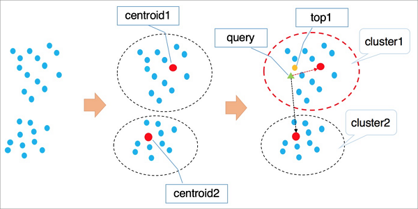
  The following figure shows how the IVFFlat algorithm works.

  

  Algorithm flow:

  1. Points in a high-dimensional space have implicit clustering properties. Clustering algorithms such as k-means are used to process the vectors so that each cluster has a centroid.

  2. When you retrieve a vector, first traverse all cluster centroids to find the n centroids nearest to the target vector.

  3. Traverse all elements in the clusters where the n centroids are located. Perform a global sort to obtain the k nearest vectors.

  Note

  • When you query cluster centroids, distant clusters are automatically excluded to speed up the query process. However, this does not guarantee that all of the top k optimal vectors are in these n clusters. This can cause a loss of precision. You can control the accuracy of the IVFFlat algorithm by adjusting the n parameter. A larger n value provides higher accuracy but requires more computation.

  • The first stage of IVFFlat and IVFADC is identical. The main difference is in the second-stage calculation. IVFADC uses product quantization to avoid traversal calculations, but this leads to a loss of precision. IVFFlat uses brute-force calculation to avoid precision loss, and the amount of computation is controllable.

• HNSW algorithm

  The Hierarchical Navigable Small World (HNSW) algorithm is suitable for scenarios with extremely large vector datasets (tens of millions or more) and strict query latency requirements (in the 10 ms range).

  HNSW is based on a navigable small world graph algorithm. It finds potential nearby points by iterating quickly through the graph. With large data volumes, the performance improvement of the HNSW algorithm is more significant than other algorithms. However, storing neighbor points consumes additional storage space. It is also difficult to improve recall accuracy by adjusting simple parameters beyond a certain threshold.

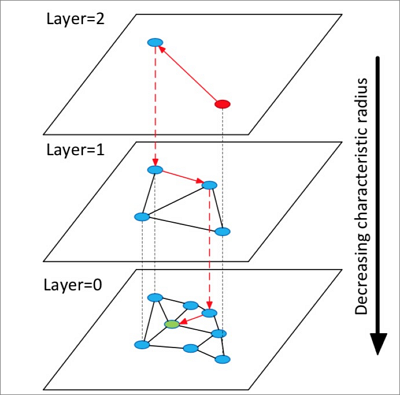
  The following figure shows how the HNSW algorithm works.

  

  Algorithm flow:

  1. Construct a multilayer graph. Each layer is a summary of the layer below it and acts as a skip list for the lower layer, similar to a highway.

  2. Start the query from a randomly selected point in the top layer.

  3. Search its neighbors. Store them in a fixed-length dynamic list in order of their distance from the target. In each subsequent search, retrieve points from the dynamic list in order. Search their neighbors, and insert these newly discovered neighbors into the dynamic list. After each insertion, sort the dynamic list and keep the top k elements. If the list changes, continue the search. Iterate until a stable state is reached. Then, use the first point in the dynamic list as the entry point for the next layer.

  4. Repeat step 3 until you reach the bottom layer.

  Note

  The HNSW algorithm builds a multilayer graph based on the single-layer graph of the NSW algorithm. It performs a nearest neighbor search in the graph, which can achieve a higher query acceleration ratio than clustering algorithms.

Both algorithms are suitable for specific business scenarios. For example, IVFFlat is ideal for high-precision image comparison, while HNSW is suited for retrieval in search and recommendation applications. We will continue to integrate leading industry algorithms into PASE.

Use PASE

1. Create the PASE extension. You can run the following command:

   CREATE EXTENSION pase;

2. Calculate vector similarity. You can calculate vector similarity using one of the following two constructor methods:

   • Calculate using the PASE data type constructor

     Example

     SELECT ARRAY[2, 1, 1]::float4[] <?> pase(ARRAY[3, 1, 1]::float4[]) AS distance;
     SELECT ARRAY[2, 1, 1]::float4[] <?> pase(ARRAY[3, 1, 1]::float4[], 0) AS distance;
     SELECT ARRAY[2, 1, 1]::float4[] <?> pase(ARRAY[3, 1, 1]::float4[], 0, 1) AS distance;

     Note

     • The <?> is an operator for the pase data type. It calculates the similarity between the vector on the left and the vector on the right. The left vector must be of the float4[] data type, and the right vector must be of the pase data type.

     • The pase type is a data type defined in the extension. It can have up to three constructors. In the third example, float4[], 0, 1 is used: The first parameter is a float4[] array that represents the right vector. The second parameter has no specific function in this context and can be set to 0. The third parameter specifies the similarity metric: 0 indicates Euclidean distance, and 1 indicates inner product.

     • The dimensions of the left and right vectors must be the same. Otherwise, an error is reported.

   • Calculate using the string constructor

     Example

     SELECT ARRAY[2, 1, 1]::float4[] <?> '3,1,1'::pase AS distance;
     SELECT ARRAY[2, 1, 1]::float4[] <?> '3,1,1:0'::pase AS distance;
     SELECT ARRAY[2, 1, 1]::float4[] <?> '3,1,1:0:1'::pase AS distance;

     Note

     Both the string constructor and the PASE data type constructor calculate the similarity between two vectors. The difference is that the string constructor uses a colon (:) as a separator. In the third example, 3,1,1:0:1 is used: The first parameter represents the right vector. The second parameter has no specific function in this context and can be set to 0. The third parameter specifies the similarity metric: 0 indicates Euclidean distance, and 1 indicates inner product.

3. Create an index. You can create an index using one of two algorithms:

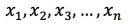
   Note

   If you use the PASE vector index with inner product or cosine as the similarity metric, you must normalize the vectors. For an original vector , it must satisfy: . After normalization, the inner product and cosine values are the same.

   • Create an index using the IVFFlat algorithm

     Example

     CREATE INDEX ivfflat_idx ON vectors_table
     USING
       pase_ivfflat(vector)
     WITH
       (clustering_type = 1, distance_type = 0, dimension = 256, base64_encoded = 0, clustering_params = "10,100");

     The following table describes the parameters.

     Parameter	Description
     clustering_type	The type of clustering operation that the IVFFlat algorithm performs on vector data. This parameter is required. Valid values: 0: External clustering. Loads an external centroid file specified by the clustering_params parameter. 1: Internal clustering. A clustering operation is first performed internally during index building. The k-means algorithm is used, which is controlled by the clustering_params parameter. For new users, we recommend internal clustering.
     distance_type	The similarity metric. The default value is 0. Valid values: 0: Euclidean distance. 1: Inner product. To use this metric, you must normalize the vectors. The order of inner product values is the reverse of the order of Euclidean distance values. Currently, only Euclidean distance is supported. To use inner product, you must normalize the vectors and then use the method described in the Appendix.
     dimension	The vector dimensions. This parameter is required. The maximum value is 512.
     base64_encoded	Specifies whether the data is Base64-encoded. The default value is 0. Valid values: 0: The vector type is represented by float4[]. 1: The vector type is represented by a Base64-encoded string of float[].
     clustering_params	For external clustering, this parameter specifies the path of the centroid file. For internal clustering, this parameter specifies the clustering parameters. The format is clustering_sample_ratio,k. This parameter is required. clustering_sample_ratio: The sampling ratio for clustering, with 1000 as the denominator. The value must be an integer from (0, 1000]. For example, a value of 1 indicates that the data in the table is sampled at a ratio of 1/1000 for k-means clustering. A larger value provides higher query accuracy but longer index creation time. We recommend that the total number of sampled data entries does not exceed 100,000. k: The number of cluster centroids. A larger value provides higher query accuracy but longer index creation time. We recommend a value from [100, 1000].

   • Create an index using the HNSW algorithm

     Example

     CREATE INDEX hnsw_idx ON vectors_table
     USING
       pase_hnsw(vector)
     WITH
       (dim = 256, base_nb_num = 16, ef_build = 40, ef_search = 200, base64_encoded = 0);

     The following table describes the parameters.

     Parameter	Description
     dim	The vector dimensions. This parameter is required. The maximum value is 512.
     base_nb_num	The number of neighbors for each node in the graph. This parameter is required. A larger value provides higher query accuracy but slower index building and a larger index size. We recommend a value from [16-128].
     ef_build	The heap length during index building. This parameter is required. A longer heap provides better results but slower index creation. We recommend a value from [40,400].
     ef_search	The heap length during a query. This parameter is required. A longer heap provides better results but lower query performance. You can specify this at query time. The default value is 200.
     base64_encoded	Specifies whether the data is Base64-encoded. The default value is 0. Valid values: 0: The vector type is represented by float4[]. 1: The vector type is represented by a Base64-encoded string of float[].

4. Run a query. You can run a query using one of two indexes:

   • Query using an IVFFlat index

     Example

     SELECT id, vector <#> '1,1,1'::pase as distance
     FROM vectors_ivfflat
     ORDER BY
     vector <#> '1,1,1:10:0'::pase
     ASC LIMIT 10;

     Note

     • The <#> is the operator for the IVFFlat index.

     • The vector index is used in the ORDER BY statement. Ascending (ASC) sort is supported.

     • The pase data type has three parts separated by colons (:). In the example 1,1,1:10:0: The first part is the query vector. The second part is a query parameter for IVFFlat. The value can range from (0, 1000]. A larger value provides higher query accuracy but lower query performance. We recommend that you determine the optimal value based on your data and debugging. The third part is the similarity metric for the query: 0 indicates Euclidean distance, and 1 indicates inner product. To use inner product, you must normalize the vectors. The order of inner product values is the reverse of the order of Euclidean distance values.

   • Query using an HNSW index

     Example

     SELECT id, vector <?> '1,1,1'::pase as distance
     FROM vectors_ivfflat
     ORDER BY
     vector <?> '1,1,1:100:0'::pase
     ASC LIMIT 10;

     Note

     • The <?> is the operator for the HNSW index.

     • The vector index is used in the ORDER BY statement. Ascending (ASC) sort is supported.

     • The pase data type has three parts separated by colons (:). In the example 1,1,1:10:0: The first part is the query vector. The second part is a query parameter for HNSW. The value can range from (0, ∞). A larger value provides higher query accuracy but lower query performance. We recommend that you determine the optimal value based on your data and debugging. We recommend starting with an initial value of 40. The third part is the similarity metric for the query: 0 indicates Euclidean distance, and 1 indicates inner product. To use inner product, you must normalize the vectors. The order of inner product values is the reverse of the order of Euclidean distance values.

Appendix

• Example of inner product calculation

  The following example uses an HNSW index. An example of the CREATE FUNCTION statement is as follows:

  CREATE OR REPLACE FUNCTION inner_product_search(query_vector text, ef integer, k integer, table_name text) RETURNS TABLE (id integer, uid text, distance float4) AS $$
  BEGIN
      RETURN QUERY EXECUTE format('
      select a.id, a.vector <?> pase(ARRAY[%s], %s, 1) AS distance from 
      (SELECT id, vector FROM %s ORDER BY vector <?> pase(ARRAY[%s], %s, 0) ASC LIMIT %s) a
      ORDER BY distance DESC;', query_vector, ef,  table_name,  query_vector, ef, k);
  END
  $$
  LANGUAGE plpgsql;

  Note

  For normalized vectors, the inner product is equal to the cosine. Therefore, you can use the method above to calculate the cosine value.

• Custom centroid file for an IVFFlat index

  This is an advanced feature. You must upload a centroid file to a specified path on the server and use it as an index parameter to build the index. For more information about the parameters, see the IVFFlat index parameter description table. The file format is as follows:

  Vector dimensions|Number of centroids|Set of centroid vectors

  Example

  3|2|1,1,1,2,2,2

References

• Product Quantization for Nearest Neighbor Search

  Herve Jégou, Matthijs Douze, and Cordelia Schmid. Product quantization for nearest neighbor search.

• Efficient and robust approximate nearest neighbor search using Hierarchical Navigable Small World graphs

  Yu. A. Malkov and D. A. Yashunin. Efficient and robust approximate nearest neighbor search using Hierarchical Navigable Small World graphs.