GeoSOT geographic grid model based on
GanosBase's GeoSOT geographic grid engine provides grid-based 3D path planning for unmanned aerial vehicle (UAV) applications in environments modeled with digital elevation models (DEMs), digital surface models (DSMs), and oblique photography.
Key concepts
A geographic grid divides the Earth's surface into a hierarchy of polygonal cells. Each cell is encoded with a unique identifier, enabling spatial positioning and feature attribution within a consistent framework. The 3D variant extends this encoding to the height dimension alongside latitude and longitude.
GanosBase supports two geographic grid types:
-
GeoSOT — A discrete, multi-scale location identification system developed based on a Chinese Earth subdivision theory. Used for 3D path planning in this guide.
-
H3 — A two-dimensional hexagonal grid developed by Uber. For details, see the H3 geographic grid capabilities documentation.
GanosBase also supports degenerated grid computation, which uses compact grid combinations to represent spatial ranges efficiently. The built-in geographic grid index accelerates grid encoding queries and aggregation.
How it works
The path planning pipeline consists of five stages. Each stage uses dedicated GanosBase functions:
| Stage | What happens | Key functions |
|---|---|---|
| 1. Import | Load OSGB oblique photography data from OSS into PolarDB | ST_ImportOSGB |
| 2. Convert | Convert tiles to GLB format via an intermediate SfMesh type | ST_ImportGLB, ST_AsGLB, ST_YupToZup, ST_Translate, ST_SetSrid, ST_Flatten, ST_Transform |
| 3. Build grid | Encode geometry as a GeomGrid obstacle array | ST_As3DGrid |
| 4. Assign costs | Set travel costs for non-passable areas and risk zones | ST_SetCost, ST_CostUnion, ST_MatchGridLevel |
| 5. Plan path | Calculate the optimal 3D grid path between two points | ST_3DGridPath |
Core functions
ST_SetCost
Sets the travel cost for a grid array representing an obstacle. Obstacles can be physical structures (such as buildings) or spatial constraints (such as radar scan areas or wind fields). Convert the obstacle's spatial range to a grid array before calling this function.
Cost conventions:
-
-1— non-passable (hard block) -
1— default passable (no penalty) -
Any positive integer greater than 1 — passable with a penalty (used for risk zones)
When a risk-zone grid overlaps a non-passable grid, the non-passable cost takes precedence.
ST_3DGridPath
Calculates the optimal 3D grid path between a start point and an end point, given a bounding box and an array of cost-assigned grid sets. Supports multiple path algorithms, movement modes, and distance calculation methods.
Parameters in the example:
-
algorithm:astar(A* algorithm) -
movement:crossorstrict_octothorpe -
distance:euclidean
All geometry inputs to ST_3DGridPath and the grid filter queries must use the EPSG:4490 spatial reference system.
ST_MatchGridLevel
Determines the highest grid level appropriate for your terrain elevation data resolution. Do not use a grid level higher than this value in path calculations, as it would exceed the precision of the underlying data.
ST_CostUnion
Merges multiple obstacle grid cost arrays into a single input for path planning. Where grids overlap, the maximum cost is applied.
Grid level reference
The ST_As3DGrid function accepts a grid level parameter that controls spatial resolution. Higher levels produce finer grids but increase processing time significantly.
| Level | Approximate size | Level | Approximate size | Level | Approximate size |
|---|---|---|---|---|---|
| 0 | Global | 11 | 29.6 km | 22 | 15.5 m |
| 1 | 1/4 of the Earth | 12 | 14.8 km | 23 | 7.7 m |
| 2 | — | 13 | 7.4 km | 24 | 3.9 m |
| 3 | — | 14 | 3.7 km | 25 | 1.9 m |
| 4 | — | 15 | 1.8 km | 26 | 1.0 m |
| 5 | — | 16 | 989.5 m | 27 | 0.5 m |
| 6 | 890.5 km | 17 | 494.7 m | 28 | 24.2 cm |
| 7 | 445.3 km | 18 | 247.4 m | 29 | 12.0 cm |
| 8 | 222.6 km | 19 | 123.7 m | 30 | 6.0 cm |
| 9 | 111.3 km | 20 | 61.8 m | 31 | 3.0 cm |
| 10 | 59.2 km | 21 | 30.9 m | 32 | 1.5 cm |
Always call ST_MatchGridLevel to confirm the maximum usable level for your terrain data before running path calculations.
Prerequisites
Before you begin, make sure you have:
-
A PolarDB for PostgreSQL (Compatible with Oracle) 2.0 cluster with the following minimum specifications:
-
Engine version: 2.0.14.23.1
-
CPU: 4 cores or more
-
Memory: 16 GB or more (greater than 16 GB recommended for OSGB import and computation)
-
Disk: 100 GB or more
-
GanosBase version: 6.7 or later
-
-
OSGB oblique photography data uploaded to an Object Storage Service (OSS) bucket
-
The original oblique data must include a complete
metadata.xmlfile so that the anchor point and coordinate reference system can be retrieved during import
Plan a 3D UAV path
This section demonstrates 3D path planning using oblique photography data from a park.
Test data
Step 1: Install extensions
Install the required extensions. If any statement fails, contact support for assistance.
CREATE EXTENSION IF NOT EXISTS ganos_geomgrid CASCADE;
CREATE EXTENSION IF NOT EXISTS ganos_utility CASCADE;
Step 2: Import OSGB data
Import the oblique photography data stored in OSS using ST_ImportOSGB. For the full function reference, see ST_ImportOSGB.
SELECT
  ST_ImportOSGB(
    'test_oblique',
    'OSS://<access_id>:<secret_key>@<Endpoint>/<bucket>/path_to/file',
    '{"parallel":16,"project":"building"}');
Replace the following placeholders:
| Placeholder | Description |
|---|---|
<access_id> |
Your Alibaba Cloud AccessKey ID |
<secret_key> |
Your Alibaba Cloud AccessKey Secret |
<Endpoint> |
The OSS endpoint for your region |
<bucket> |
The OSS bucket name |
Step 3: Convert tiles to GLB
Convert the target level-of-detail (LOD) tiles to GLB format using SfMesh as an intermediate type, and store the result in a temporary table.
SELECT
  ST_ImportGLB(
    'temp_glb',
    ST_AsGLB(ST_Combine(tile)),
    'temp_glb_1',
    '{"ignore_texture":true,"ignore_normal":true}'
  )
FROM test_oblique_tile WHERE lod = 19 AND project_name = 'building';Setignore_textureandignore_normaltotrueto skip unnecessary data during grid construction.
lod = 19 selects tiles at level of detail 19. Adjust this to match your data. Higher LOD values produce more accurate results but increase processing time.This example uses standard OSGB file naming (for example,Tile_+006_+004_L14_0.osgb), where the LOD can be parsed from the filename. If your data uses non-standard naming, replaceWHERE lod = 19withWHERE children IS NULLto select the leaf nodes with highest precision.
Step 4: Reproject coordinates to EPSG:4490
Oblique photography data typically uses relative coordinates anchored to a local origin. This step applies the correct absolute coordinates, establishes the CGC 2000 spatial reference system (EPSG:4490), and pre-flattens rotation matrices.
UPDATE temp_glb
SET
  gltf_data = ST_Transform(
    ST_Flatten(
      ST_SetSrid(
        ST_Translate(
          ST_YupToZup(gltf_data),
          x_off, y_off, z_off),
        srid),
      FALSE),
    4490)
FROM
  (SELECT
      srid,
      ST_X(anchor) x_off,
      ST_Y(anchor) y_off,
      ST_Z(anchor) z_off
    FROM test_oblique WHERE project_name = 'building') metadata
WHERE gltf_id = 'temp_glb_1';
This statement performs the following operations in sequence:
-
[ST_YupToZup](https://www.alibabacloud.com/help/en/polardb/polardb-for-oracle/st-yuptozup) — OSGB format uses the Y-axis as the vertical reference. This function reorients the coordinate frame to Z-up before any other transformations.
-
[ST_Translate](https://www.alibabacloud.com/help/en/polardb/polardb-for-oracle/translate-1) — Applies the anchor point offset to convert all relative coordinates to absolute coordinates.
-
[ST_SetSrid](https://www.alibabacloud.com/help/en/polardb/polardb-for-oracle/setsrid-1) — Assigns the correct spatial reference system ID from the metadata.
-
[ST_Flatten](https://www.alibabacloud.com/help/en/polardb/polardb-for-oracle/st-flatten) — Applies any embedded rotation matrices to the actual vertex coordinates, which is required before reprojection.
-
[ST_Transform](https://www.alibabacloud.com/help/en/polardb/polardb-for-oracle/transform) — Reprojects all points to EPSG:4490, the coordinate reference system used by GeoSOT grids.
This operation requires the original oblique data to include a complete metadata.xml file. Without it, the anchor point and spatial reference system cannot be retrieved.
Step 5: Build the obstacle grid
Convert the geometry to a GeomGrid array and store it in the grid table. Drop the temporary GLB table when done.
-- Create the grid table
CREATE TABLE IF NOT EXISTS building_grid
(
   id        SERIAL,
   grid      GEOMGRID,
   grid_type TEXT
);

-- Generate GeomGrid data and insert into the grid table
INSERT INTO building_grid (grid, grid_type)
SELECT grid, 'border'
FROM
  (SELECT unnest(ST_As3DGrid(gltf_data, 24, TRUE)) grid
   FROM temp_glb WHERE gltf_id = 'temp_glb_1') tmp;

-- Remove the temporary table
DROP TABLE temp_glb;
The second argument to ST_As3DGrid sets the grid level. Level 24 (~3.9 m per cell) is used here. See Grid level reference for the full size table.
Verify: Preview grid geometry
Export the grid as GLB to verify the obstacle shape before running path planning.
SELECT
  ST_AsGLB(
    ST_ZupToYup(
      ST_3DRemoveDuplicateVertex(
        ST_MergeGeomByMaterial(
          ST_Triangulate(
            ST_Translate(
              ST_Transform(
                ST_Flatten(
                  ST_Collect(
                    ST_AsMeshgeom(array (SELECT grid FROM building_grid WHERE grid_type = 'border')):: sfmesh[]),
                  TRUE
                ),
                srid
              ),
              - ST_X(anchor), - ST_Y(anchor), - ST_Z(anchor)
            )
          )
        ),
        0.1
      )
    )
  )
FROM test_oblique WHERE project_name = 'building';
This statement:
-
Converts the grid array to a MeshGeom array via ST_AsMeshGeom, then combines all elements into a single SfMesh with ST_Collect.
-
Applies pre-flattening with
ST_Flattenand reprojects to the original coordinate system with ST_Transform. -
Offsets coordinates back to a local origin with ST_Translate.
-
Triangulates the mesh with ST_Triangulate and reduces data volume with
ST_MergeGeomByMaterialand ST_3DRemoveDuplicateVertex. -
Converts from the Z-up coordinate frame back to Y-up (as required by glTF) with ST_ZupToYup, then exports as GLB with ST_AsGLB.
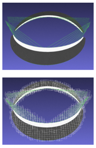
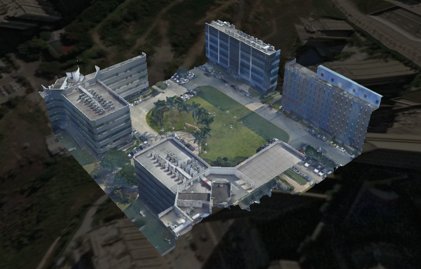
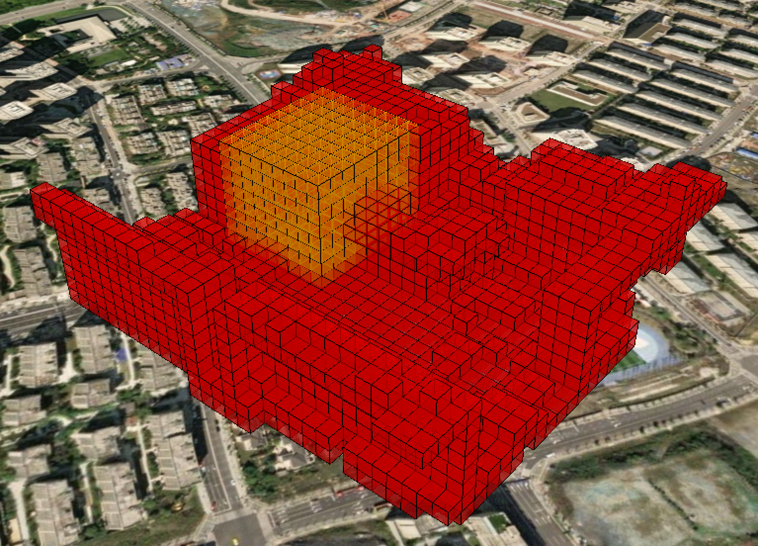
The following table compares the grid output at two different levels.
| Level | Result |
|---|---|
| Raw data | 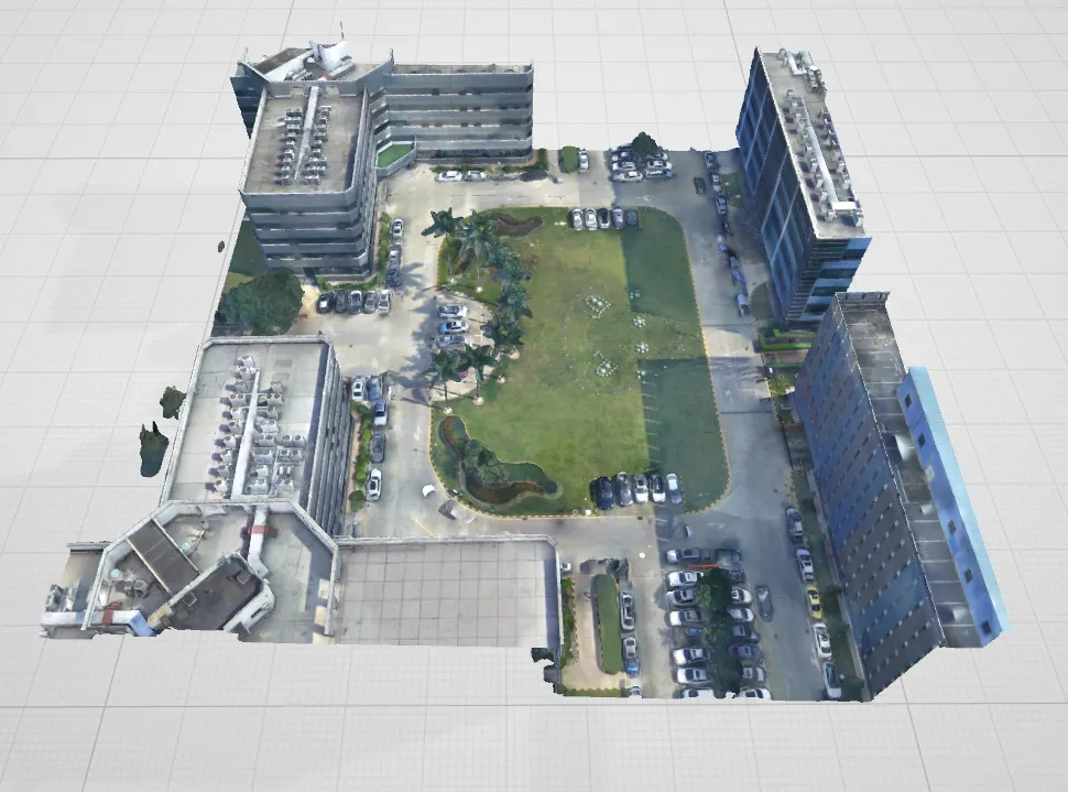 |
| Level 25 | 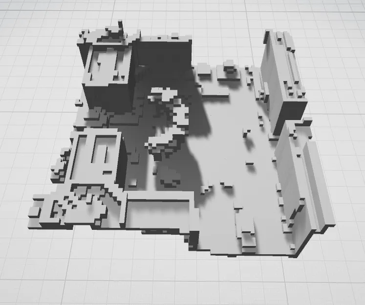 |
| Level 24 | 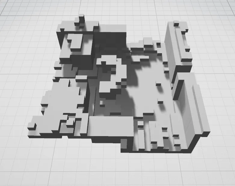 |
View grids in Cesium
Use the GridToJson helper function to generate Cesium-compatible grid data.
-- Create the helper function
CREATE OR REPLACE FUNCTION GridToJson(geomgrid[])
RETURNS json AS $$
SELECT to_json(
        array_agg(
            json_build_object('center', array_to_json(array[ST_X(center), ST_Y(center), ST_Z(center)]),
                           'size', array_to_json(array[ST_DistanceSpheroid(min_point, ST_Point(ST_X(max_point), ST_Y(min_point), 4490)), ST_DistanceSpheroid(min_point, ST_Point(ST_X(min_point), ST_Y(max_point), 4490)), z]))))
FROM
  (SELECT ST_Transform(ST_PointZ(ST_X(st_centroid(geom)), ST_Y(st_centroid(geom)), (ST_ZMax(geom) + ST_ZMin(geom)) / 2, 4490), 4479) center,
          ST_SetSrid(BOX[0]::geometry, 4490) min_point,
          ST_SetSrid(BOX[1]::geometry, 4490) max_point,
          ST_ZMax(geom) - ST_ZMin(geom) z
   FROM
     (SELECT ST_ASBox(grid) BOX, ST_AsGeometry(grid) geom
      FROM (SELECT unnest($1) grid) a)b)c $$
LANGUAGE 'sql';

-- Call GridToJson to generate the result
SELECT GridToJson(array (SELECT grid FROM building_grid WHERE grid_type = 'border'));GridToJsonconverts each grid cell's spatial reference from EPSG:4490 to EPSG:4479 when computing thecenterfield. Thesizevalues remain in the EPSG:4490 scale (latitude/longitude/height directions). Adjust theST_Transformcall if your Cesium setup requires a different coordinate reference system.
The function returns a JSON array:
[
  {
    "center": [-1583397.2647956165, 5313841.088458569, 3142388.7651142543],
    "size": [3.3600142470488144, 3.848872238575258, 3.3680849811062217]
  },
  ...
]-
center: Grid cell center in EPSG:4479. -
size: Approximate cell dimensions in the latitude, longitude, and height directions.
Load the result in Cesium with the following HTML:
<!DOCTYPE html>
<html lang="en">
<head>
  <meta charset="utf-8">
  <script src="https://cesium.com/downloads/cesiumjs/releases/1.89/Build/Cesium/Cesium.js"></script>
  <link href="https://cesium.com/downloads/cesiumjs/releases/1.89/Build/Cesium/Widgets/widgets.css" rel="stylesheet">
  <style>
    html, body, #cesium_container {
      width: 100%; height: 100%;
      margin: 0; padding: 0; overflow: hidden;
    }
  </style>
</head>
<body>
  <div id="cesium_container"></div>
  <script>
    Cesium.Ion.defaultAccessToken = YOUR_CESIUM_TOKEN
    const viewer = new Cesium.Viewer('cesium_container', ['timeline', 'animation', 'infoBox', 'navigationHelpButton'].reduce((opts, opt) => (opts[opt] = false) || opts, {}))

    // Specify the grids to display
    const grids = [{ "center": [-1583315.44750805, 5313895.98214751, 3142303.525767127], "size":...
    const add_grids = (grids, material) =>
      grids.forEach(({ center, size }) => viewer.entities.add({
          position: new Cesium.Cartesian3(...center),
          box: {dimensions: new Cesium.Cartesian3(...size),
            material, outline: true, outlineColor: Cesium.Color.BLACK}}))

    // Display grids in semi-transparent red
    add_grids(grids, Cesium.Color.RED.withAlpha(0.2))

    // Jump to the grid location
    viewer.zoomTo(viewer.entities)
  </script>
</body>
</html>
Replace YOUR_CESIUM_TOKEN with your Cesium Ion access token.
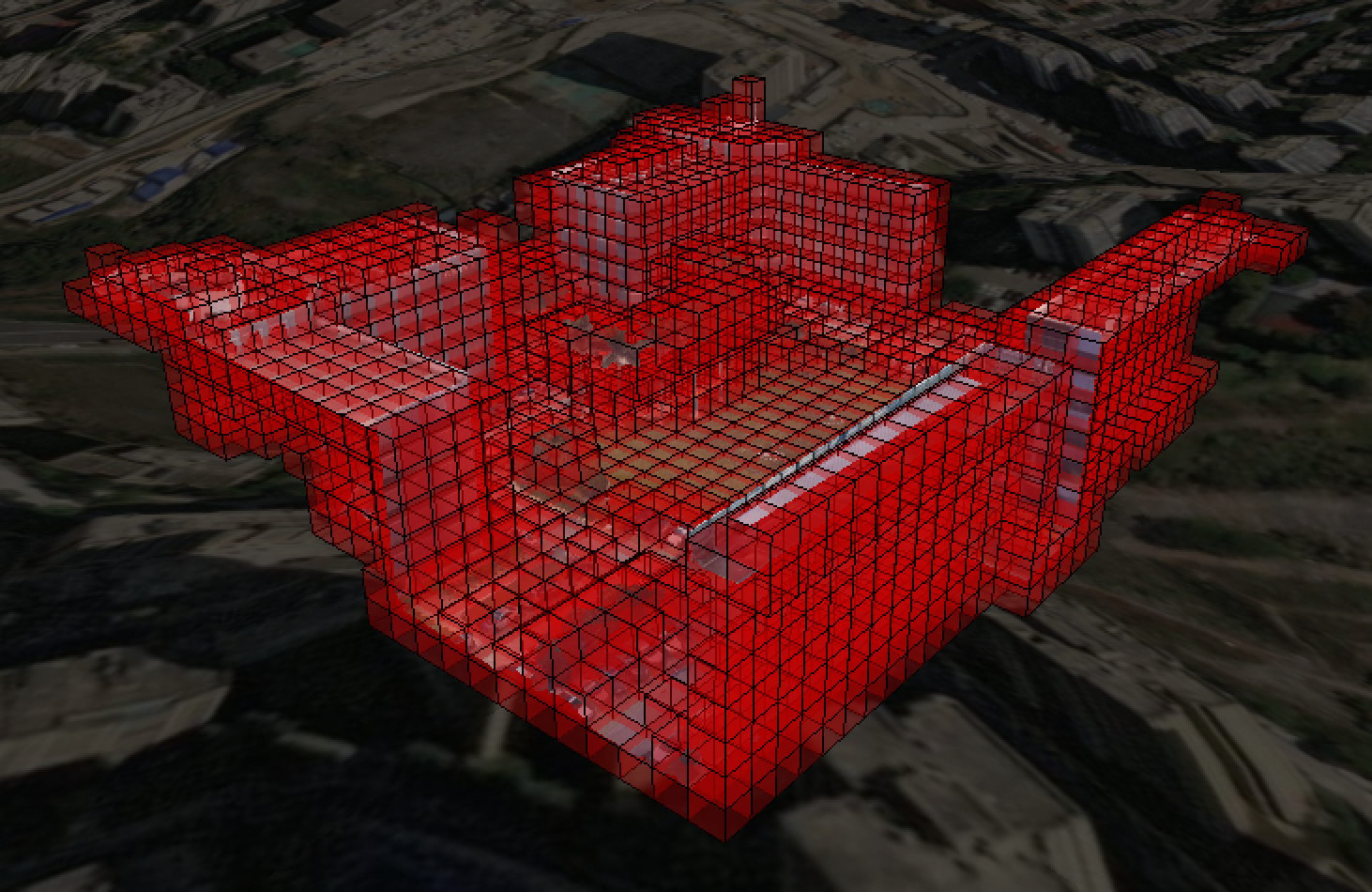
The following figure shows the level 24 grid overlaid on the oblique photography data. For the full code to load the oblique data, see Appendix.
Step 6: Run path planning
Plan a 3D path through the grid using ST_3DGridPath. The query defines the start point, end point, and a bounding box that limits the search space to relevant grids only.
-- Define start point, end point, and search bounds
WITH vals (start_p, end_p, box_range) AS (
VALUES
(
ST_PointZ(106.59182291666669, 29.70644097140958, 355.322855208642, 4490),
ST_PointZ(106.59244791666666, 29.707135415854022, 348.58669235736755, 4490),
'BOX3D(106.591788194444 29.7062326380763 341.85053662386713, 106.592899305556 29.7071701380762 362.0590251699541)' :: box3d
)),
border AS (
SELECT DISTINCT grid, grid_type
FROM building_grid, vals
WHERE
-- Filter to grids within the bounding box only.
-- All geometry inputs must use EPSG:4490.
ST_3DIntersects(ST_SetSrid(box_range :: meshgeom, 4490), grid)
OR ST_3DContains(ST_SetSrid(box_range :: meshgeom, 4490), grid)
)
SELECT ST_3DGridPath(
start_p,
end_p,
box_range,
array[ST_SetCost(array (SELECT grid FROM border WHERE grid_type = 'border'), -1)],
'{"algorithm":"astar","movement":"cross","distance":"euclidean"}'
) result
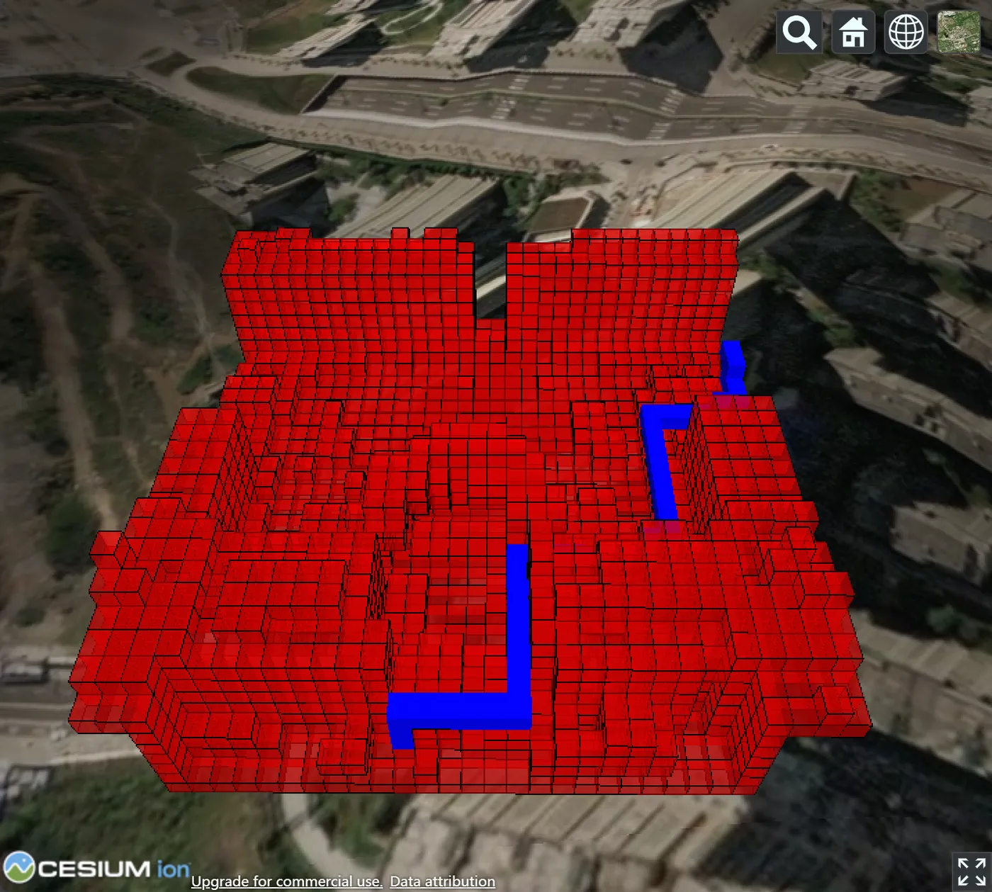
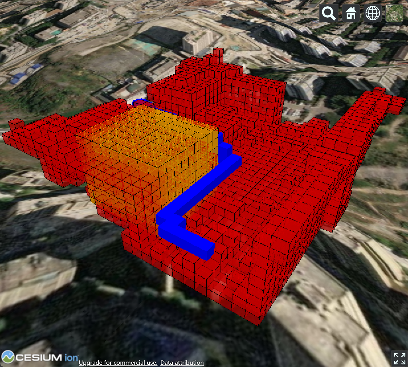
FROM vals;ST_SetCost(..., -1) marks all building grids as non-passable. The A* algorithm finds the shortest Euclidean path that avoids these cells.
Visualize the result with GridToJson in Cesium:
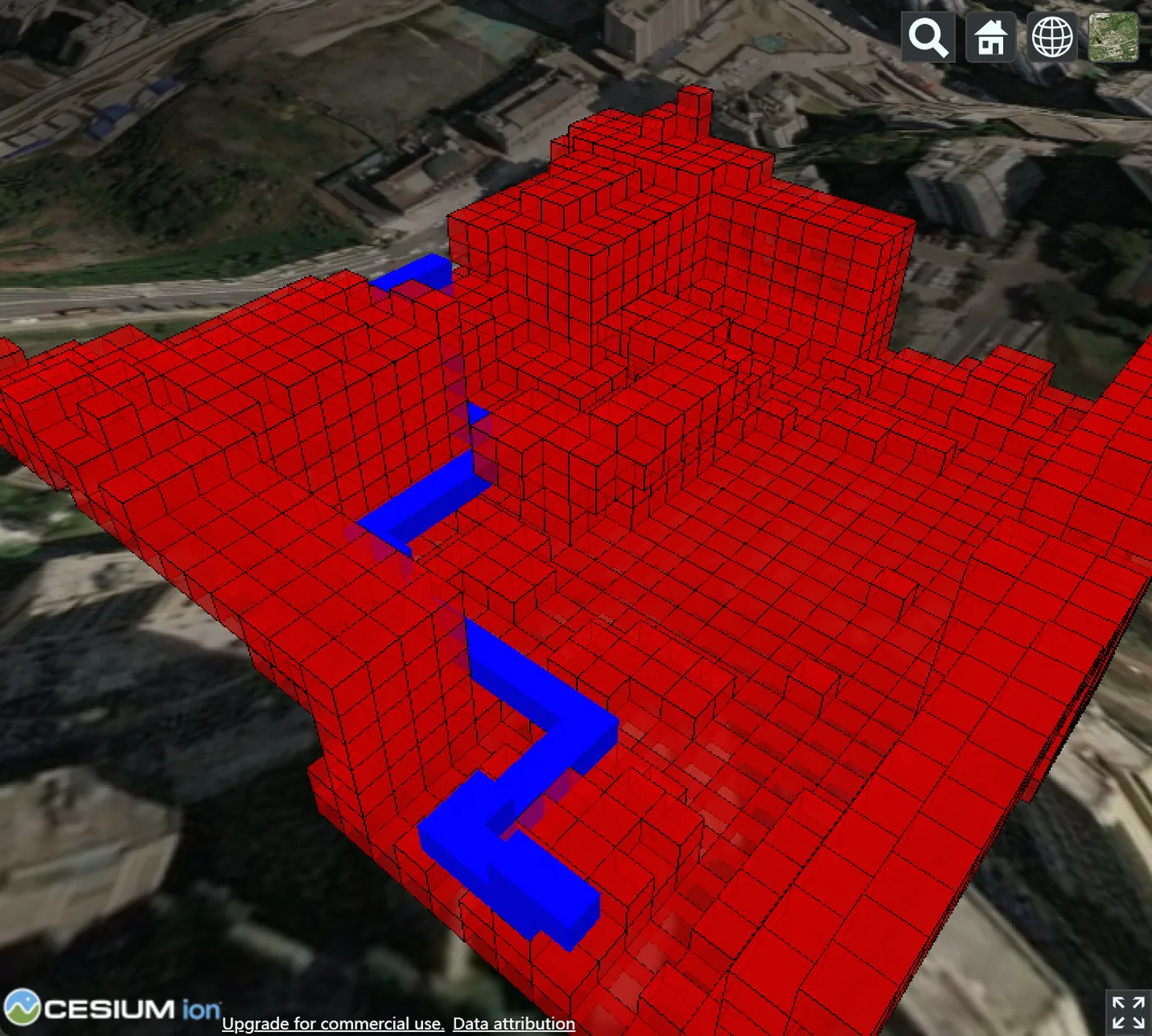
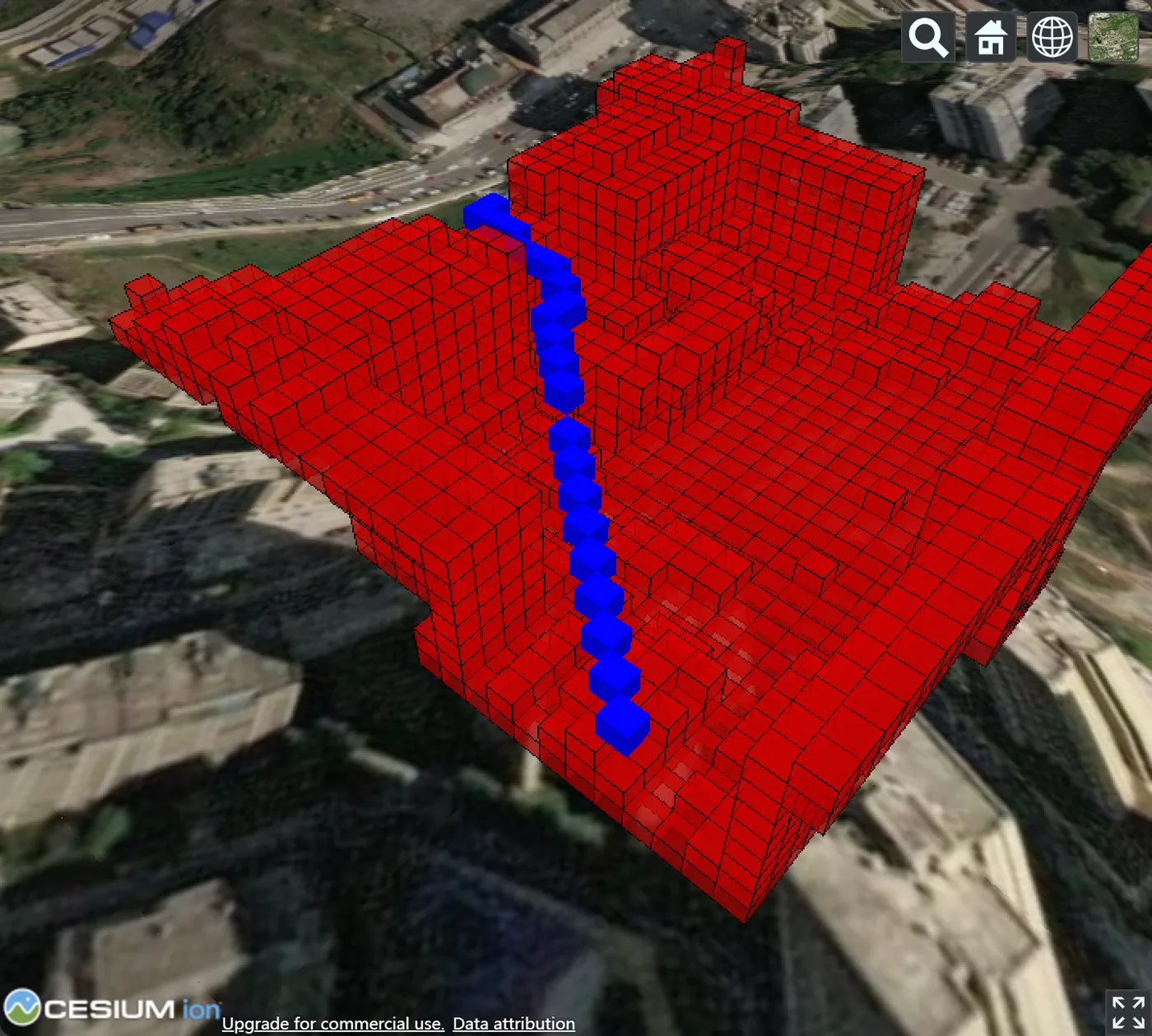
Changing the movement mode to strict_octothorpe produces a different path:
Multi-cost path planning
Assign different travel costs to different zones so the algorithm selects the path with the lowest total cost. This example adds a risk zone to the previous scenario, causing the planned path to route around it.
1. Insert the risk zone grid.
INSERT INTO building_grid (grid, grid_type)
SELECT grid, 'risk_zone'
FROM
  (SELECT unnest(ST_As3DGrid(ST_SetSrid('BOX3D(106.59192708333332 29.706614582520686 341.8505366235368, 106.59220486111111 29.706892360298472 365.4271128197744)' :: box3d :: meshgeom, 4490), 24)) grid) tmp;
The orange area in the following figure shows the risk zone:
Risk-zone grids that overlap non-passable grids are treated as non-passable.
2. Run path planning with two cost sets.
WITH vals (start_p, end_p, box_range) AS (
VALUES
(
ST_PointZ(106.59182291666669, 29.70644097140958, 355.322855208642, 4490),
ST_PointZ(106.59244791666666, 29.707135415854022, 348.58669235736755, 4490),
'BOX3D(106.591788194444 29.7062326380763 341.85053662386713, 106.592899305556 29.7071701380762 362.0590251699541)' :: box3d
)),
border AS (
SELECT DISTINCT grid, grid_type
FROM building_grid, vals
WHERE
ST_3DIntersects(ST_SetSrid(box_range :: meshgeom, 4490), grid)
OR ST_3DContains(ST_SetSrid(box_range :: meshgeom, 4490), grid)
)
-- border grids: non-passable (-1); risk_zone grids: cost 2
SELECT ST_3DGridPath(
start_p,
end_p,
box_range,
array[
ST_SetCost(array (SELECT grid FROM border WHERE grid_type = 'border'), -1),
ST_SetCost(array (SELECT grid FROM border WHERE grid_type = 'risk_zone'), 2)
],
'{"algorithm":"astar","movement":"cross","distance":"euclidean"}'
) result
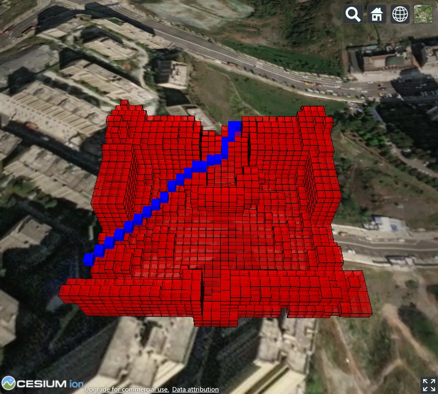
FROM vals;The A* algorithm routes around the risk zone to minimize total path cost:
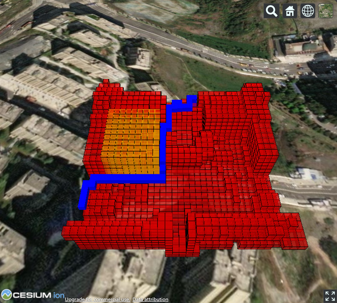
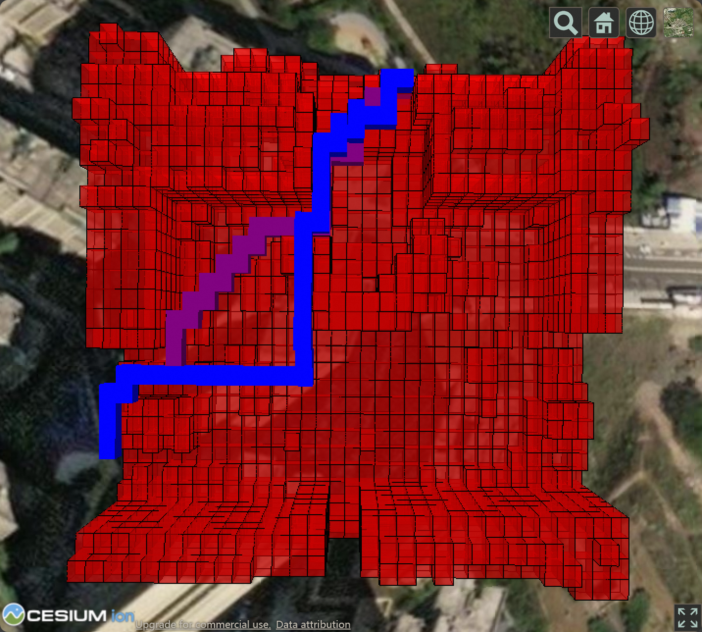
The following figure compares the path without a risk zone (purple) against the path that avoids the risk zone:
Appendix
This appendix provides a Node.js backend service that proxies 3D Tiles requests, with Cesium as the visualization frontend.
1. Create the dependency file `package.json` in your project directory.
{
  "dependencies": {
    "koa": "^2.14.2",
    "koa-router": "^12.0.0",
    "koa-send": "^5.0.1",
    "pg": "^8.10.0"
  }
}
2. Run `npm install`, then create `index.js` in the same directory.
const Koa = require('koa');
const Send = require('koa-send');
const Router = require('koa-router');
const router = new Router()
const { Pool } = require('pg');
const pool = new Pool({ user: <YOUR_USER>, host: <YOUR_HOST>, database: <YOUR_DB_NAME>, port: <YOUR_PORT> });

const TABLE_NAME = 'test_osgb'
const PROJECT_NAME = 'prj1'

router.get('/', (_) => Send(_, '/index.html'))

/* Get metadata of the current project */
router.get('/project', async (ctx) => {
  const sql = `SELECT (REGEXP_MATCHES(ST_ASTEXT(ST_TRANSFORM(ANCHOR,4326)), 'POINT Z \\((.*?)\\)'))[1] _ANCHOR, PROJECT_ID FROM ${TABLE_NAME} WHERE PROJECT_NAME='${PROJECT_NAME}';`
  const { rows: [{ _anchor, project_id }] } = await pool.query(sql)
  const anchor = _anchor.split(' ').map(x => parseFloat(x))
  const url = `/tileset/${project_id}/${project_id}`
  ctx.body = { url, anchor }
})

router.get('/tileset/:project_id/:uid', async (ctx) => {
  const { params: { project_id, uid } } = ctx
  const sql = `SELECT TILESET FROM ${TABLE_NAME}_TILESET WHERE PROJECT_ID=$1::UUID AND UID=$2::UUID;`
  const { rows: [{ tileset }] } = await pool.query(sql, [project_id, uid])
  ctx.body = tileset
})

router.get('/b3dm/:project_id/:uid', async (ctx) => {
  const { params: { project_id, uid } } = ctx
  const sql = `SELECT ST_ASB3DM(TILE) TILE FROM ${TABLE_NAME}_TILE WHERE PROJECT_ID=$1::UUID AND UID=$2::UUID;`
  const { rows: [{ tile }] } = await pool.query(sql, [project_id, uid])
  ctx.body = tile
})

new Koa().use(router.routes()).listen(5500, '0.0.0.0');
Replace <YOUR_USER>, <YOUR_HOST>, <YOUR_DB_NAME>, and <YOUR_PORT> with your PolarDB connection details.
3. Create `index.html` in the same directory.
<!DOCTYPE html>
<html lang="en">

<head>
  <meta charset="utf-8">
  <script src="https://cesium.com/downloads/cesiumjs/releases/1.89/Build/Cesium/Cesium.js"></script>
  <link href="https://cesium.com/downloads/cesiumjs/releases/1.89/Build/Cesium/Widgets/widgets.css" rel="stylesheet">
  <style>
    html, body, #cesium_container {
      width: 100%; height: 100%;
      margin: 0; padding: 0; overflow: hidden;
    }
  </style>
</head>

<body>
  <div id="cesium_container"></div>
  <script>
    Cesium.Ion.defaultAccessToken = <SET_YOUR_OWN_TOKEN_HERE>
    const disable_opt = ['timeline', 'animation', 'infoBox', 'navigationHelpButton']
      .reduce((opts, opt) => (opts[opt] = false) || opts, {})
    const viewer = new Cesium.Viewer('cesium_container', disable_opt)
    fetch('/project')
      .then(res => res.json())
      .then(({ anchor, url }) => {
        const position = Cesium.Cartesian3.fromDegrees(...anchor)
        const modelMatrix = Cesium.Transforms.eastNorthUpToFixedFrame(position)
        const tileset = new Cesium.Cesium3DTileset({ url, modelMatrix })
        tileset.readyPromise.then(() => viewer.zoomTo(tileset))
        viewer.scene.primitives.add(tileset)
      })
  </script>
  </div>
</body>

</html>
4. Start the service and open the viewer.
node index.jsOpen http://localhost:5500 in your browser to view the oblique photography data.