Systems generate anomalies — sudden CPU spikes, network floods, unexpected state transitions. Catching them before they escalate requires a model that monitors your metrics in real time and flags deviations before they become incidents. This tutorial walks you through building and evaluating a binary classification model on PAI (Machine Learning Platform for AI) to detect system anomalies from monitoring logs.
Prerequisites
Before you begin, make sure you have:
Familiarity with machine learning fundamentals, particularly feature engineering and binary classification algorithms
More than 1,000 labeled data records (each labeled
anomalyornormal)One to two days available for end-to-end development
An active PAI workspace with access to Visualized Modeling (Designer)
The workspace is associated with MaxCompute resources. For more information, see Quick start - Preparations.
Dataset
This tutorial uses a system-level monitoring log dataset with 22,544 records, of which 9,711 are labeled as anomalies. The following figure shows sample data.
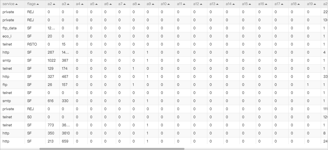
Parameter | Description |
| Protocol used for the network connection. Valid values: |
| Service protocol. Valid values: |
| Connection status. Valid values: |
| System metrics. |
| Label field. |
How the pipeline works
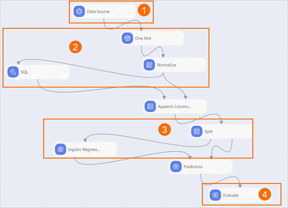
The pipeline runs in four stages:
Data ingestion — Imports the labeled monitoring log dataset.
Feature engineering — Prepares the data for training:
One Hot Encoding converts string-type features (such as
protocol_typeandservice) to numeric values.Normalization scales all numeric values to the range 0–1, so no single metric dominates the model due to its magnitude.
SQL Script converts the
classlabel to a binary integer:anomaly→1,normal→0. The SQL statement is:SELECT (CASE class WHEN 'anomaly' THEN 1 ELSE 0 END) AS class FROM ${t1};
Model training — Trains a logistic regression binary classification model on the prepared data to distinguish normal events from anomalies.
Evaluation — Measures model quality using the area under the curve (AUC), Kolmogorov-Smirnov (KS) statistic, and F1 score.
Build and run the pipeline
Open Visualized Modeling (Designer)
Log on to the PAI console.
In the left-side navigation pane, click Workspaces, then click the workspace you want to use.
In the left-side navigation pane, choose Model Training > Visualized Modeling (Designer).
Create the pipeline from a template
On the Preset Templates tab, find the Abnormal Behavior Risk Control template and click Create.
In the Create Pipeline dialog box, review the parameters.
The Data Storage parameter specifies the Object Storage Service (OSS) bucket path where the pipeline stores temporary data and model artifacts generated during the run.
Click OK. The pipeline is created in about 10 seconds.
On the Pipelines tab, double-click Abnormal Behavior Risk Control to open the pipeline. The canvas displays the pipeline components, as shown in the following figure.
Run the pipeline
In the upper-left corner of the canvas, click
 to start the run.
After the pipeline finishes, right-click the Evaluate component and select Visual Analysis.
In the Evaluate dialog box, click the Index data tab to view the model evaluation metrics.
Evaluate the model
The evaluation results are as follows:
KS: 0.8821572036692878
AUC: 0.9834216679657054
F1 Score: 0.9510219822599307
Negative Samples: 1950
Positive Samples: 2566
Total Samples: 4516
The AUC value is greater than 0.9, which indicates that the prediction accuracy of the model is higher than 90%.
Once the model meets your accuracy threshold, deploy it to an online prediction service to enable nearline risk control on live system metrics.