Platform For AI:Scorecard credit scoring

Prerequisites

• You have created a workspace. For more information, see Create and manage workspaces.

• You have associated a MaxCompute resource with the workspace. For more information, see Create and manage workspaces.

Dataset

This pipeline uses an open-source dataset from a foreign organization (Download dataset) with 30,000 records. The dataset includes user information such as gender, education, marital status, age, credit card transaction history, and billing statements.

Scorecard credit scoring

1. Go to the Machine Learning Designer page.

   1. Log on to the PAI console.

   2. In the left-side navigation pane, click Workspaces. On the Workspaces page, click the name of the workspace that you want to manage.

   3. In the left-side navigation pane, choose Model Training > Visualized Modeling (Designer).

2. Build the pipeline.

   1. On the Designer page, click the Preset Templates tab.

   2. On the Preset Templates page, click Create under Credit Consumption Analysis Based on Scorecard.

   3. In the Create Pipeline dialog box, configure the parameters. You can keep the default settings.

      The Data Storage parameter specifies an OSS Bucket path to store temporary data and models generated during pipeline runs.

   4. Click Confirm.

      The pipeline is created in about 10 seconds.

   5. On the Pipelines tab, double-click Credit Consumption Analysis Based on Scorecard to open the pipeline.

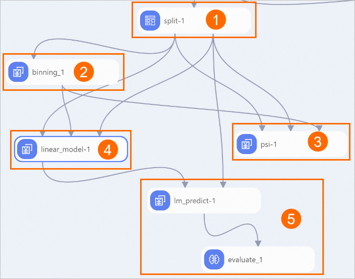
   6. The system automatically builds a pipeline from the preset template, as shown below.

      

      Area	Description
      ①	Splits the input dataset into a training dataset and a prediction dataset.
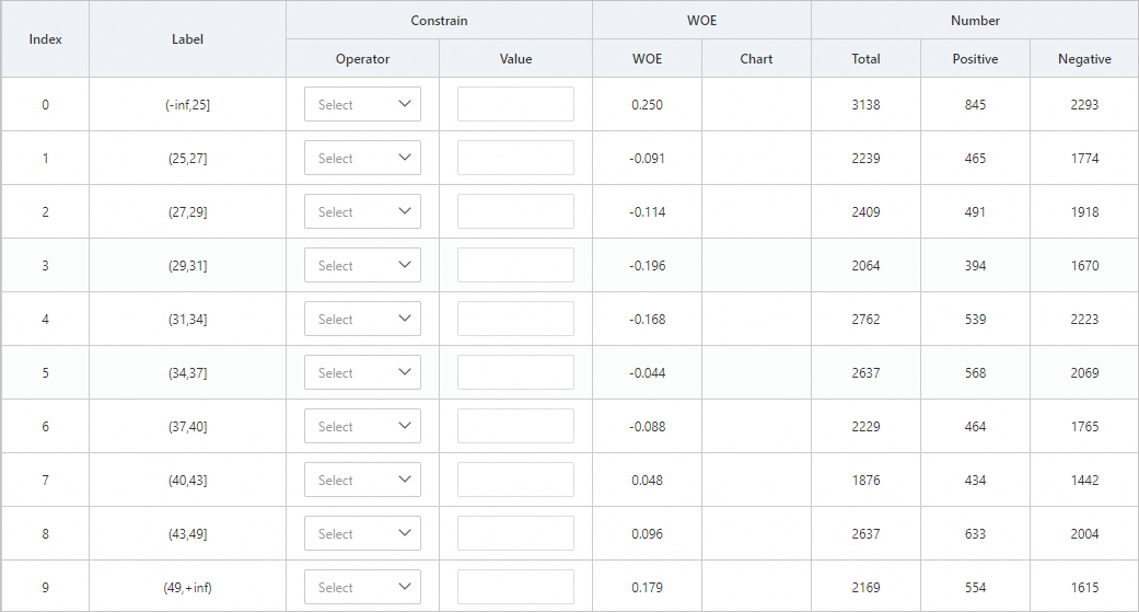
      ②	The Binning component is similar to one-hot encoding and can map data to high-dimensional features based on the data distribution. For example, for the age field, the Binning component can perform binning operations based on the distribution of data in different intervals. After the workflow completes, you can right-click the Binning-1 component and select Binning. In the Binning-1 configuration panel, click the name (age) to view the details. The result is shown in the following figure.After the workflow completes, you can right-click the Binning-1 component, and on the shortcut menu, select View Data > Binning Result Output to view that each field is binned into multiple intervals, as shown in the following figure.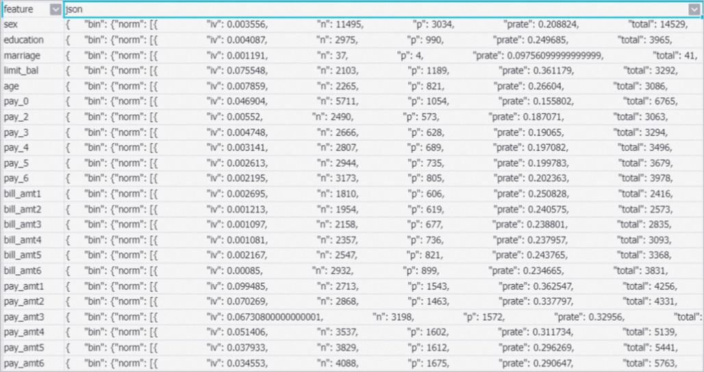
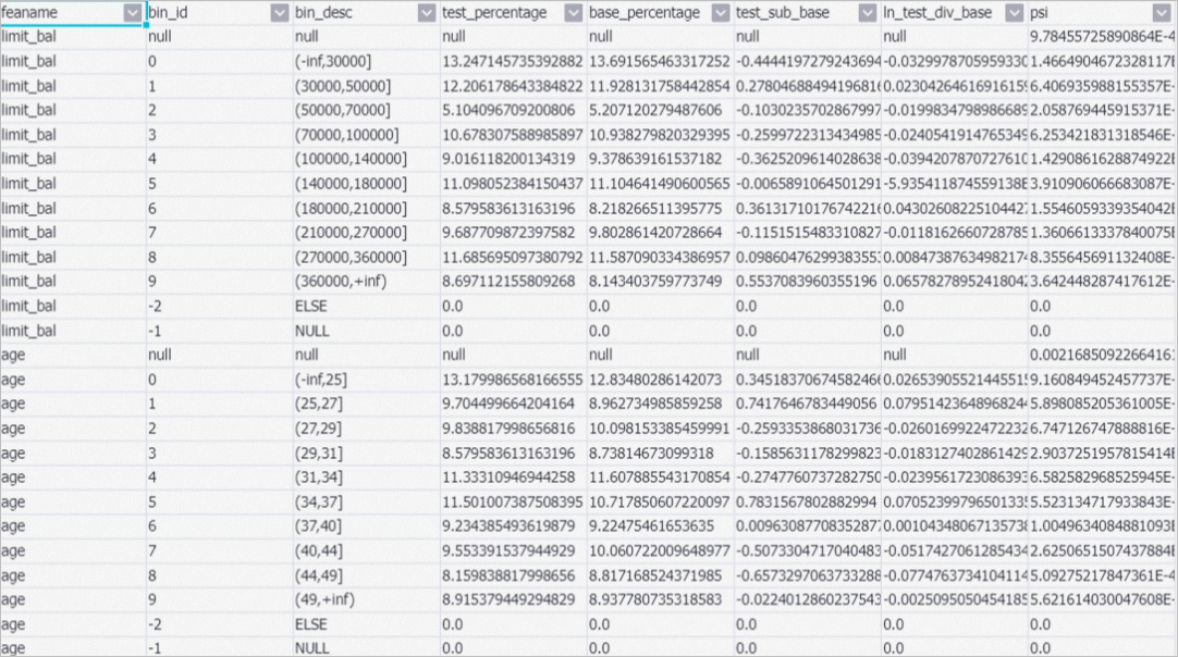
      ③	This component compares the sample stability before and after the split and binning, and returns the population stability index (PSI) for each feature. After the pipeline runs, you can right-click the PSI-1 component and choose View Data > Output to view the details, as shown in the following figure. The population stability index (PSI) is a key metric for measuring the shift in a sample distribution and assessing its stability. The total PSI for a feature is the sum of the PSI values from each of its bins. Generally, a PSI value below 0.1 indicates an insignificant change. A PSI value between 0.1 and 0.25 indicates a moderate change. A PSI value above 0.25 indicates a significant change that requires special attention.
      ④	Scorecard training. After the pipeline runs, you can right-click the Scorecard Training-1 component and choose View Data > Output Training Result Table to view the training results, as shown in the following figure.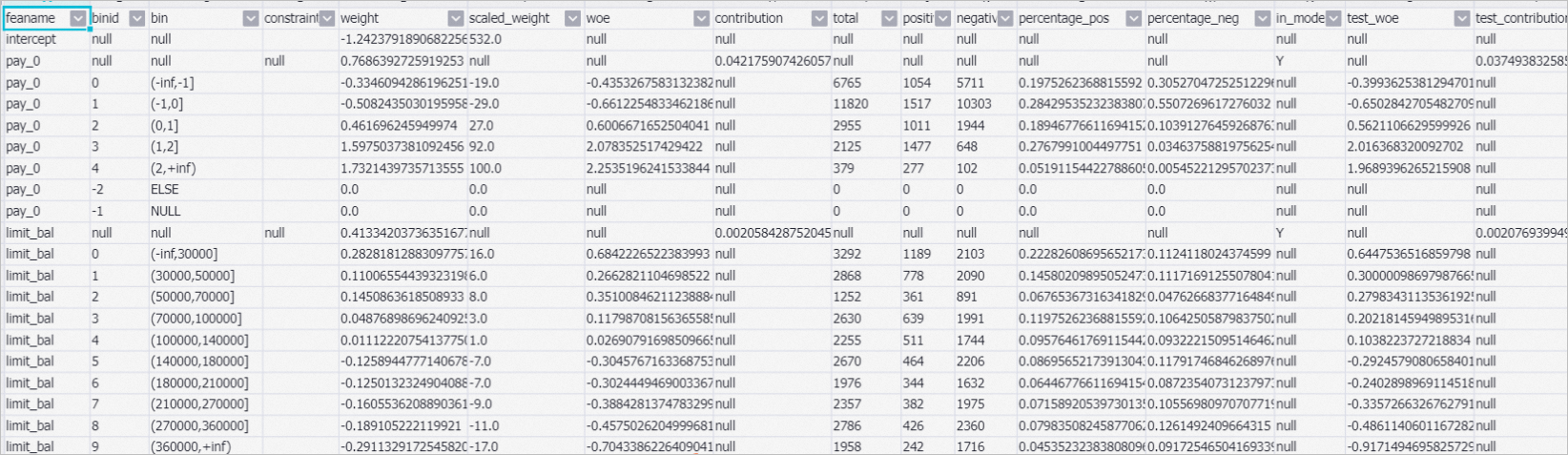A scorecard's essence is representing complex model weights with business-friendly scores. The key parameters in the results are as follows: weight: Specifies the original weight value. Scaled_weight: The score change metric. For example, for the pay_0 feature, if the feature value is in the (-1,0] interval, the score is reduced by 29. If the feature value is in the (0,1] interval, the score is increased by 27. contribution: The impact of each feature on the result. A larger value indicates a greater impact.
      ⑤	Predicts the credit score for each user and evaluates the model's performance.

3. Run the pipeline and view the results.

   1. Click the run icon at the top of the canvas.

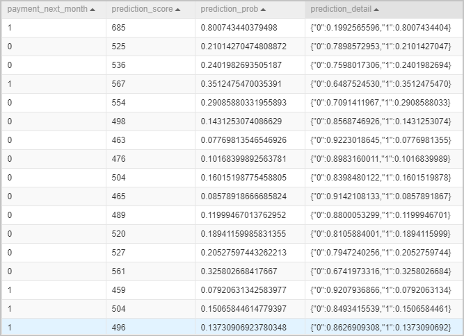
   2. After the pipeline finishes running, right-click the Scorecard Prediction-1 component on the canvas and choose View Data > Output from the shortcut menu to view the credit score for each user.