Create a custom pipeline in PAI Designer - Platform For AI

Prerequisites

PAI is activated and a workspace is created. Activate and create a default workspace.
The workspace is associated with a MaxCompute resource. Quick Start - Prerequisites.

Step 1: Create a pipeline

Open Machine Learning Designer, select a workspace, and in the upper-right corner, click New Pipeline. Enter a pipeline name and click OK.

Parameter	Description
Workflow name	Custom workflow name.
Workflow data storage	OSS Bucket storage path for temporary data and models generated during runtime. If not configured, uses default workspace storage. For each run, Designer automatically creates a temporary folder at `workflow_storage_path/task_ID/node_ID`, simplifying OSS storage path configuration for each component and enabling easier data management.
Visibility	Visible to Me: Creates workflow in the My Pipelines folder, visible only to you and workspace administrators. Visible to Current Workspace: Creates workflow in the Pipelines Visible to Workspaces folder, visible to everyone in the workspace.

Step 2: Prepare and preprocess data

Prepare and preprocess training data before building the model.

Prepare data

Add Source/Target components to read data from MaxCompute, OSS, or other sources. Component Reference: Source/Target. This example uses Read Table to read a public heart disease dataset from PAI. Heart Disease Data Set.

Select a Source/Target component to read data.

In the left component list, click Source/Target and drag Read Table to the canvas. A Read Table-1 node is created.
Configure the source table.

Select Read Table-1 on the canvas. In the configuration pane on the right, enter a MaxCompute table name in Table Name. For this example, enter pai_online_project.heart_disease_prediction.
Switch to the Fields tab to view field details.

Preprocess data

The binary logistic regression component requires DOUBLE or BIGINT input. Preprocess the dataset with data type conversion for model training.

Convert non-numeric fields to numeric types.
1. Search for SQL script and drag it to the canvas. An SQL script-1 node is created.
2. Connect Read Table-1 to the t1 input port of SQL script-1.
3. Configure the node.
  
  Click SQL script-1. In the configuration pane, enter the following SQL. The Input source on the Parameters tab is t1.
```
select age,
(case sex when 'male' then 1 else 0 end) as sex,
(case cp when 'angina' then 0  when 'notang' then 1 else 2 end) as cp,
trestbps,
chol,
(case fbs when 'true' then 1 else 0 end) as fbs,
(case restecg when 'norm' then 0  when 'abn' then 1 else 2 end) as restecg,
thalach,
(case exang when 'true' then 1 else 0 end) as exang,
oldpeak,
(case slop when 'up' then 0  when 'flat' then 1 else 2 end) as slop,
ca,
(case thal when 'norm' then 0  when 'fix' then 1 else 2 end) as thal,
(case status  when 'sick' then 1 else 0 end) as ifHealth
from  ${t1};
```
4. Click Save in the upper-left corner of the canvas.
5. Right-click the SQL script-1 component and select Run from Root Node To Here to debug and run the pipeline.
  
  Nodes run sequentially. A icon appears on each node after successful execution.
  
  Note
  You can also click (Run) in the upper-left corner of the canvas to run the entire pipeline. For complex pipelines, run individual nodes to simplify debugging. If a run fails, right-click the failed node and select View Log to troubleshoot.
6. After the run, right-click the destination node, such as SQL script-1, and select to verify the output.
Convert all fields to the DOUBLE data type.

Drag data type conversion to the canvas and connect it after SQL script-1. On the Set fields tab, click Select fields under Columns to convert to double and select all fields.
Normalize features to the [0, 1] range.

Drag normalization to the canvas and connect it after data type conversion-1. Select all fields on the Set fields tab.
Split data into training and test sets.

Drag split to the canvas and connect it after normalization-1. This component outputs two tables.

By default, data splits at a 4:1 ratio. Adjust Splitting ratio on the Parameters tab. Split.
Right-click data type conversion-1 and select Run from Here to run the remaining nodes.

Step 3: Train a model

Heart disease prediction is a binary classification problem — each sample indicates sick or healthy. Use the binary logistic regression component to build the model.

Drag the Binary Logistic Regression component to the canvas and connect it to the split-1 node's Output Table 1 port.
Configure the node.

Click binary logistic regression-1. On the Set fields tab, set Label column to ifhealth and Feature columns to all remaining columns. Binary Logistic Regression.

Note
To deploy the model in Step 6: Deploy the model (optional), you must select binary logistic regression and check Generate PMML file on the Set fields tab.
Run the node.

Step 4: Make predictions

Drag prediction to the canvas. Connect its inputs to binary logistic regression-1 and the Output Table 2 port of split-1.
Click prediction-1. On the Set fields tab, set Columns to be kept to ifhealth and Feature columns to all columns except ifhealth.
Run the prediction node and view results.

Right-click the prediction node and choose View Data > Output of Prediction Result.

The output contains: ifhealth (actual label, 1.0 or 0.0), prediction_result (predicted result), prediction_score (confidence score), and prediction_detail (per-class probabilities in JSON).

Step 5: Evaluate the model

Drag binary classification evaluation to the canvas and connect it after prediction-1.
Click binary classification evaluation-1. On the Set fields tab, set Original label column to ifhealth.
Run the evaluation node.

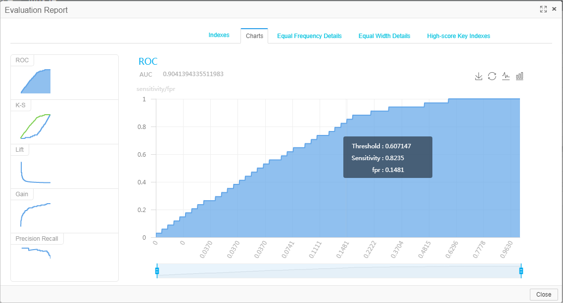
Right-click binary classification evaluation and select Visual Analysis to view evaluation metrics.

Step 6: Deploy the model (optional)

Machine Learning Designer integrates with Elastic Algorithm Service (EAS). After training, prediction, and evaluation, deploy the model to EAS as an online service.

After the pipeline runs, click Model List, select a model, and click Deploy to EAS.
Confirm the configuration. Deploy a model as an online service.

Model file and Processor type are preconfigured. Adjust other parameters as needed.
Click Deploy.

The service is deployed when Service status changes from Creating to Running.

Important
To avoid unnecessary charges, click Stop in Actions when the service is no longer needed.

Platform For AI:Custom pipeline