OpenSearch:Introduction to vectors

Introduction to vector retrieval

In the current information age, information has expanded beyond text to include multimodal information such as images, videos, and audio. Multimodal information can convey what text cannot express, such as colors, shapes, motion dynamics, sounds, and spatial relationships.

At the same time, the modalities of information in various fields have also changed significantly:

In such multimodal scenarios, information is divided into two major categories: structured and unstructured.

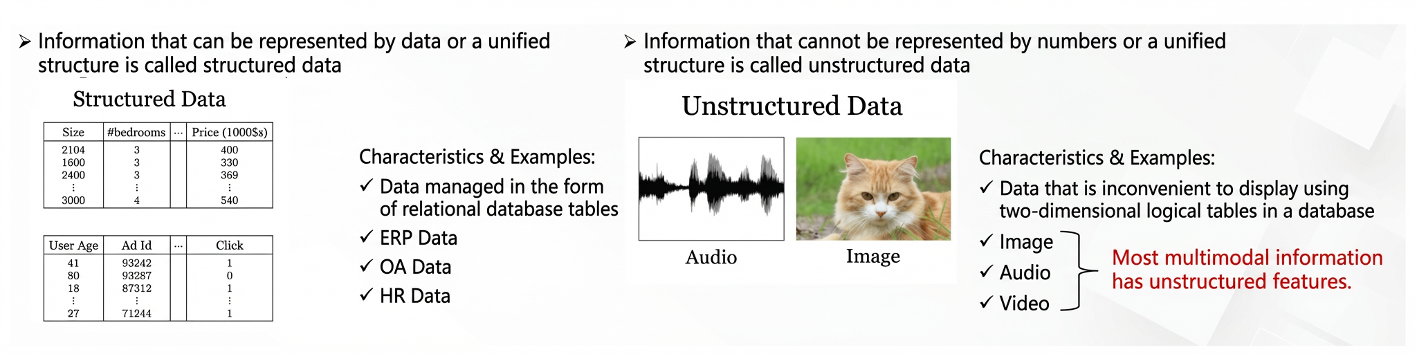
Unstructured data is often difficult for computers to understand. Traditional retrieval based on text tokenization can no longer meet the search requirements of various fields. Vectors solve this problem effectively.

So what are vectors, and how is retrieval performed by using vectors?

Unstructured data generated in the physical world is converted into structured multi-dimensional vectors. These vectors are used to represent entities and the relationships between entities.

Then, the distances between vectors are calculated. In most cases, a shorter distance indicates a higher similarity. The top results with the highest similarity are recalled to complete the retrieval.

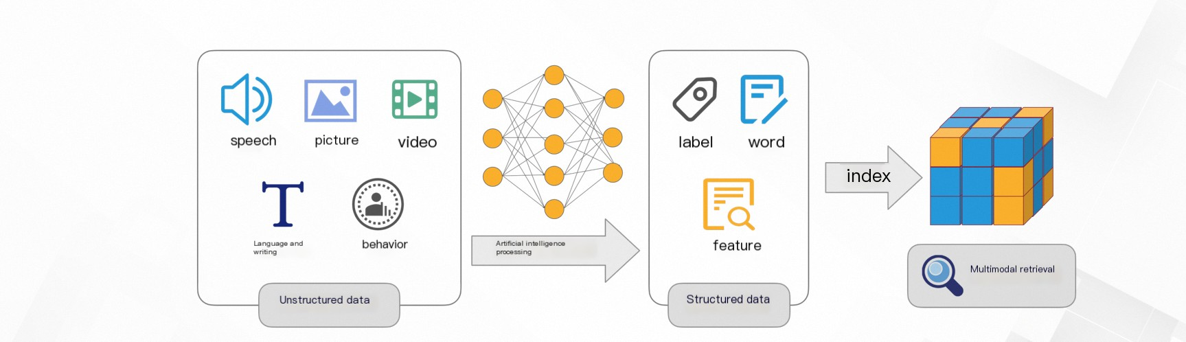
Vector retrieval algorithms

linear

The linear algorithm performs linear calculations on all vector data.

Scenarios: A recall rate of 100% is required.

Disadvantages: Efficiency is low for large amounts of data, and resource consumption (CPU and memory) is high.

Clustering algorithms

Quantized Clustering

Introduction:

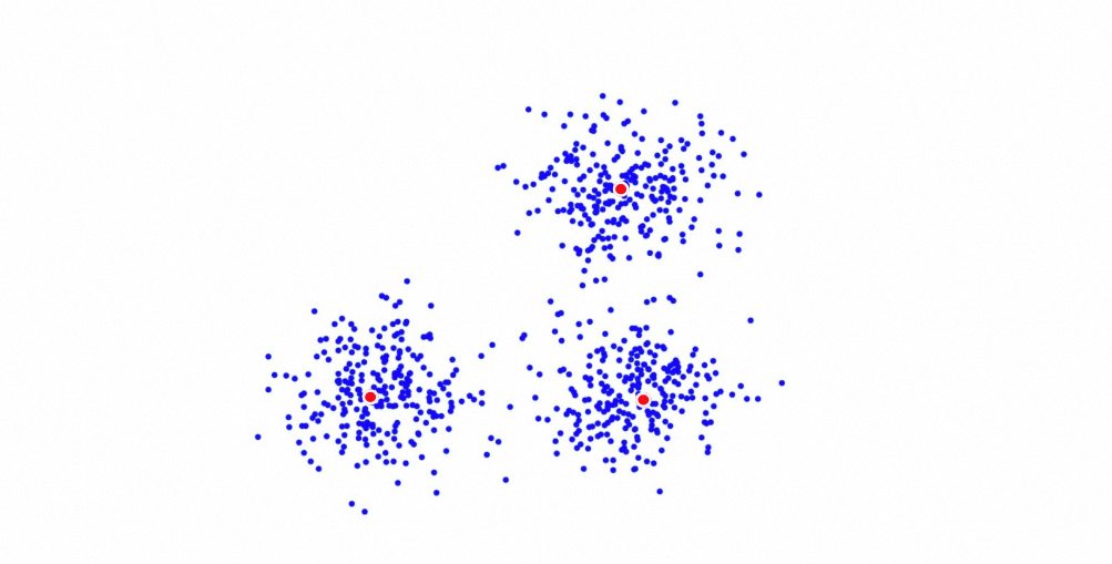
Quantized Clustering (QC) is a vector retrieval algorithm developed by Alibaba based on k-means clustering. QC first clusters vector documents into n centroids and assigns each document to its nearest centroid to build n inverted lists. The n centroids and their corresponding inverted lists make up the main content of a QC index. During retrieval, the distances between the query and some of the centroids are calculated, and the multiple nearest centroids are selected. Then, the distances between the query and the documents in the inverted lists of these centroids are calculated, and the top k nearest documents are returned.

In particular, QC supports fp16 and int8 numeric quantization, which can reduce the index size and improve retrieval performance. However, quantization may compromise the recall performance. You can determine whether to configure quantization based on your business requirements.

The QC algorithm is suitable for real-time data scenarios, or scenarios in which GPU resources are available and low latency is required.

Parameter tuning:

Quantized Clustering configuration

Performance comparison:

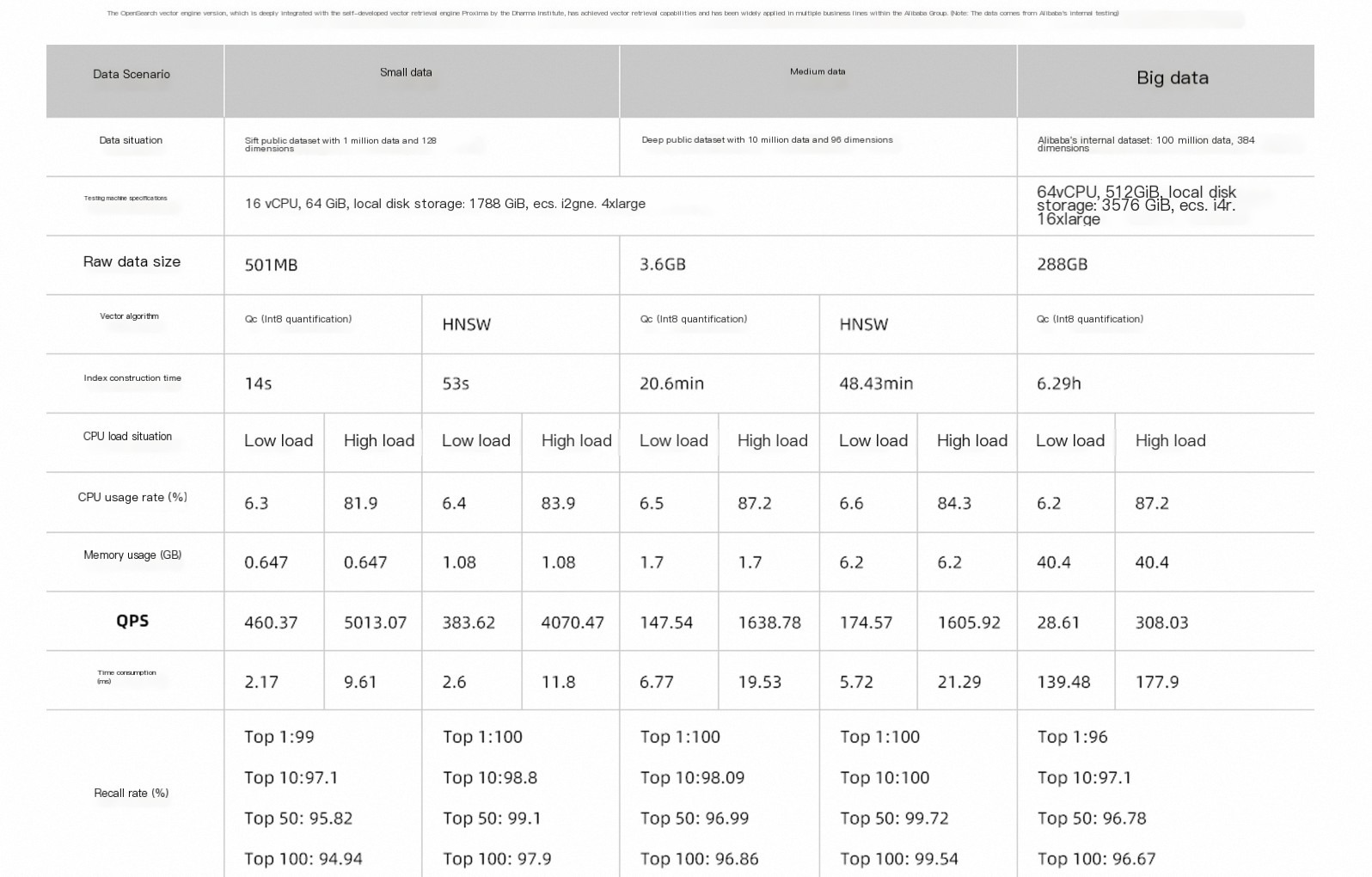
HNSW (Hierarchical Navigable Small World)

Introduction:

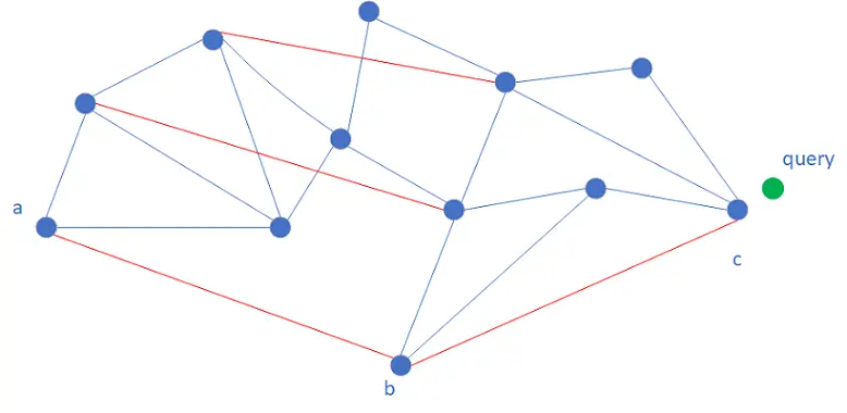
Hierarchical Navigable Small World (HNSW) is a vector retrieval algorithm based on a proximity graph. HNSW first builds a proximity graph in which edges are created between vectors that are close to each other. The vectors and their neighbor information make up the main content of an HNSW index. During retrieval, traversal starts from the entry node. The distances between the query and all neighbors of the entry node are calculated, and the nearest neighbor is selected as the next node to traverse. The traversal iterates until it converges, and then the retrieval stops. Convergence means that none of the neighbors of the current node is closer to the query than the nearest node that has already been retrieved.

To accelerate convergence, HNSW borrows the query logic of skip lists and builds a multi-layer proximity graph structure. Retrieval proceeds from the top layer down. The retrieval logic of each layer is roughly the same, except for some differences in layer 0. After the traversal on layer k converges to a node, that node is used as the entry node of layer k-1, and the traversal continues on layer k-1. Compared with the graph on layer k-1, the graph on layer k contains sparser nodes with longer distances between them. This allows larger steps and faster iterations when traversing layer k.

Parameter tuning:

HNSW (Hierarchical Navigable Small World) configuration

QGraph algorithm

Introduction:

Quantized Graph (QGraph) is an improved algorithm based on HNSW that is developed by OpenSearch. During index building, QGraph automatically quantizes the raw data of users and then builds a graph index. Compared with the HNSW algorithm, the QGraph algorithm can effectively reduce the index size and save memory. The index can be reduced to as little as 1/8 of its original size. In addition, by leveraging CPU instruction optimizations for integer computation, QGraph delivers several times the performance of HNSW. After quantization, vectors become less distinguishable, so the recall rate of QGraph is lower than that of HNSW. In real-world scenarios, you can mitigate this impact by recalling more results.

QGraph supports int4, int8, and int16 quantization of data. Different quantization levels have different impacts on the memory usage of vector indexes, query performance, and recall rate. In most cases, the fewer bits the integer type has, the less memory the vector index occupies, the higher the performance, and the lower the recall rate. Due to limitations of the underlying CPU instruction set, the performance and recall rate of int16 quantization are almost the same as those without quantization.

Parameter tuning:

QGraph (Quantized Graph) configuration

CAGRA algorithm

Introduction:

CUDA ANN GRAph-based (CAGRA) is a vector retrieval algorithm based on a proximity graph. It is optimized for NVIDIA GPUs and is suitable for scenarios with high concurrency and batch requests.

Unlike the HNSW algorithm, the CAGRA algorithm builds a proximity graph with only one layer to support parallel computing. During a query, the algorithm maintains an ordered candidate set while iterating. In each iteration, the best top K nodes in the candidate set are selected as search starting points, and their neighbors are used to try to update the candidate set. The iterations continue until all top K nodes in the candidate set have been used as search starting points. At this point, the algorithm is considered to have converged.

The CAGRA implementation includes two strategies: single-CTA and multi-CTA. Single-CTA maps the query of a single vector to a single thread block for execution and is more efficient when the batch size is large. Multi-CTA uses multiple thread blocks to execute the query of a single vector. When the batch size is small, multi-CTA makes better use of the parallel computing capability of GPUs and achieves a higher recall rate. However, when the batch size is large, its throughput is lower than that of the single-CTA strategy. During actual calls, the optimal algorithm is automatically selected based on the workload.

Parameter tuning:

CAGRA configuration

Vector distance types

Vector retrieval calculates the similarity between vectors and returns the top K vectors with the highest similarity. In this process, the similarity between vectors is obtained by calculating distances. In most cases, a smaller score indicates a shorter distance between vectors, and a larger score indicates a longer distance.

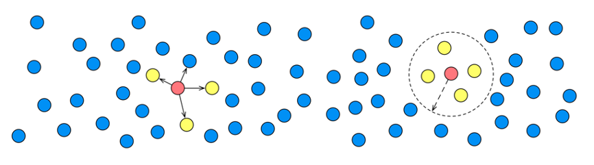
Different vector spaces define different distance metrics to calculate the distances between vectors. OpenSearch Vector Search Edition supports the following metrics: Euclidean metric and inner product metric.

Euclidean distance (SquareEuclidean)

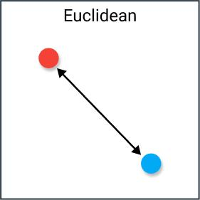
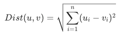
Euclidean distance is the straight-line distance between two vectors in space. As one of the most commonly used distance metrics, Euclidean distance is calculated as the square root of the sum of the squared differences between the coordinates of two vectors. A smaller Euclidean distance indicates that the two vectors are more similar. The Euclidean distance is calculated by using the following formula:

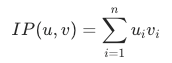
Inner product distance (InnerProduct)

The inner product is the dot product, or scalar product, of two vectors. A larger inner product indicates a higher similarity. It is calculated by multiplying the elements at corresponding positions of two vectors and summing the products. The inner product metric is common in search and recommendation scenarios. In most cases, whether to use the inner product metric depends on whether the algorithm uses an inner product model. The inner product is calculated by using the following formula:

Selection of vector retrieval algorithms