This topic describes how to analyze MaxCompute fee distribution based on usage records. You can obtain and analyze your MaxCompute bills to prevent unexpected costs, maximize resource utilization, and reduce expenses.
Background information
MaxCompute is a cloud-native big data computing service developed by Alibaba Cloud. Formerly known as ODPS, it is an enterprise-grade, SaaS-based, AI-native data warehouse that delivers high cost efficiency, multi-model computing, enterprise-grade security, and AI-driven capabilities. You can use either the subscription or pay-as-you-go billing method for MaxCompute computing resources. MaxCompute charges you daily per project. Bills are generated before 06:00 the next day. For more information about billable items and billing methods, see Billing items and billing methods.
Alibaba Cloud publishes information about MaxCompute bill fluctuations—typically fee increases—during data development or before product releases. You can analyze these fluctuations and optimize jobs in your MaxCompute projects. You can download usage records for all Alibaba Cloud paid services from the Expenses and Costs console. For more information about obtaining and downloading bills, see View billing details.
Step 1: Download usage records
Go to the Usage Records page to download daily usage records and understand fee generation. For example, identify which jobs generate daily storage and computing fees.
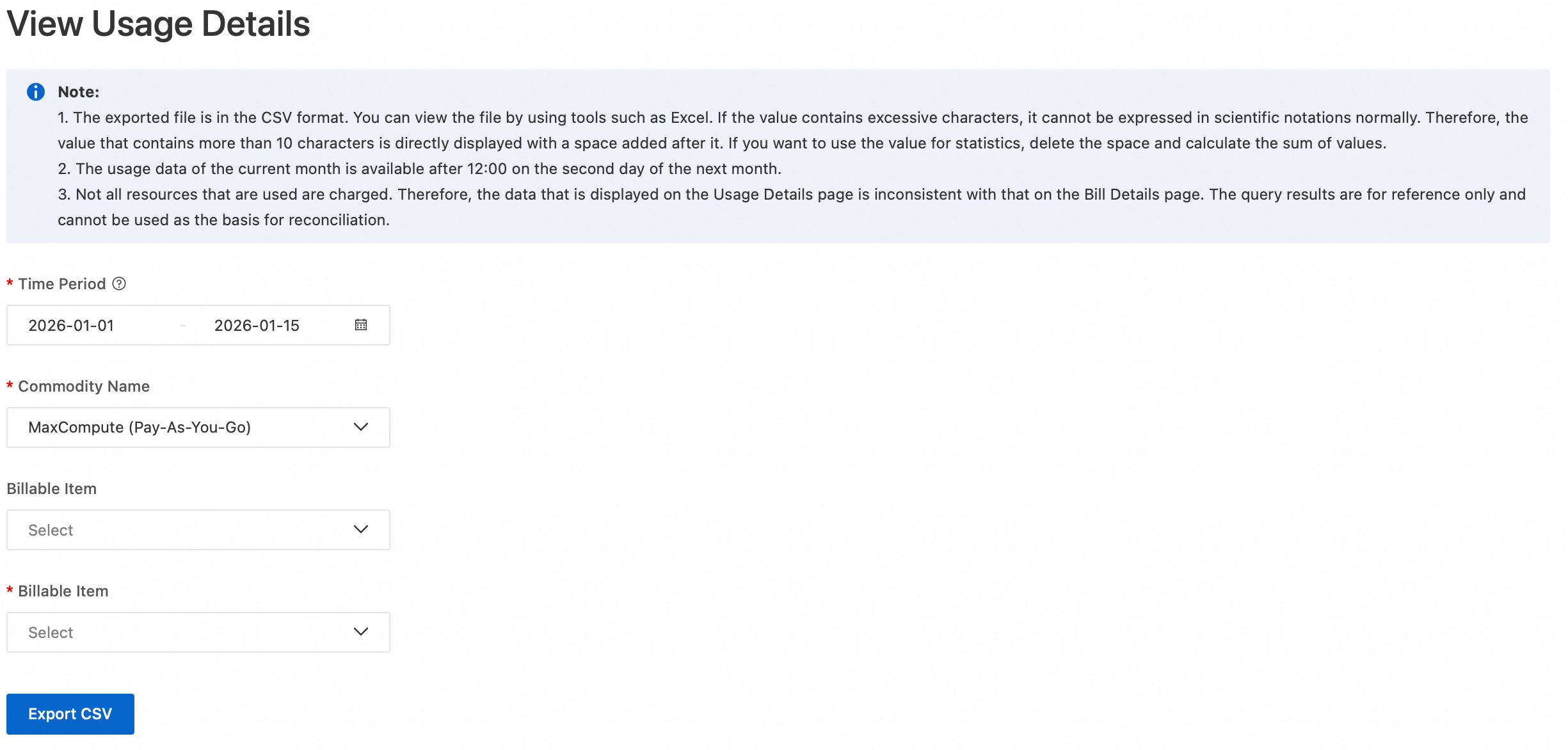
Click Export CSV. After a short wait, go to the Export Records page to download the usage records.
Parameter descriptions
Time Period: Click to select the start and end times.
If a job starts on December 1 and ends on December 2, set the start time to December 1 to include the job in the downloaded usage records. However, the consumption record appears in the December 2 bill.
Commodity Name:
MaxCompute(Subscription)
MaxCompute (Pay-as-you-go)
Billable Item: You can select as needed.
Billable Item
ODPSDataPlus:
If you have only purchased subscription projects for MaxCompute in a region, the usage of pay-as-you-go billing items, such as storage and download, is metered within the subscription project.
Before April 25, 2024, if you had both subscription and pay-as-you-go MaxCompute projects enabled in Hong Kong (China) or a region outside China, the default compute quota was associated with the subscription project. This quota also covered the measurement details for pay-as-you-go storage and download billing items. In such cases, you can obtain the measurement details for the pay-as-you-go project’s default compute quota by querying MaxCompute (Pay-As-You-Go).
ODPS_QUOTA_USAGE: Metering records for elastically reserved computing resources and dedicated Tunnel resources.
MaxCompute (Pay-as-you-go): Metering records for pay-as-you-go billing items, such as computing, storage, and download.
Time Unit: Hour, by default.
Step 2 (Optional): Upload usage records to MaxCompute
If you want to analyze usage records using MaxCompute SQL, follow this step to upload them to MaxCompute. Skip this step if you plan to use Excel only.
Create a MaxCompute table named
maxcomputefeeusing the MaxCompute client (odpscmd). Sample statement:CREATE TABLE IF NOT EXISTS maxcomputefee ( projectid STRING COMMENT 'Project ID' ,feeid STRING COMMENT 'Metering ID' ,meteringtime STRING COMMENT 'MeteringTime' ,type STRING COMMENT 'Metering type, such as Storage, ComputationSQL, or DownloadEx' ,starttime STRING COMMENT 'Start time' ,storage BIGINT COMMENT 'Storage (bytes)' ,endtime STRING COMMENT 'End time' ,computationsqlinput BIGINT COMMENT 'SQL input (bytes)' ,computationsqlcomplexity DOUBLE COMMENT 'SQL complexity' ,uploadex BIGINT COMMENT 'Internet upload (bytes)' ,download BIGINT COMMENT 'Internet download (bytes)' ,cu_usage DOUBLE COMMENT 'MR/Spark compute (core*second)' ,Region STRING COMMENT 'Region' ,input_ots BIGINT COMMENT 'Input from Tablestore (bytes)' ,input_oss BIGINT COMMENT 'Input from OSS (bytes)' ,source_id STRING COMMENT 'DataWorks node ID' ,source_type STRING COMMENT 'Specification type' ,RecycleBinStorage BIGINT COMMENT 'Recycle bin storage (bytes)' ,JobOwner STRING COMMENT 'Job owner' ,Signature STRING COMMENT 'SQL job signature' );Field descriptions:
Project ID: List of MaxCompute projects for your Alibaba Cloud account or the Alibaba Cloud account associated with the current RAM user.
Metering ID: Billing ID. This is the task ID for storage, computing, upload, or download tasks. For SQL tasks, it is the InstanceID. For upload or download tasks, it is the Tunnel SessionId.
Metering type: Storage, ComputationSql, UploadIn, UploadEx, DownloadIn, or DownloadEx. Only items shown in red are billed.
Storage (bytes): Storage volume read per hour, in bytes.
Start time or End time: Measured based on actual job execution time. Only storage is sampled hourly.
SQL input (bytes): Input data volume for each SQL execution, in bytes.
SQL complexity: SQL complexity, one of the SQL billing factors.
Internet upload (bytes) or Internet download (bytes): Data volume uploaded or downloaded over the Internet, in bytes.
MR/Spark compute (core*second): Billable hours for MapReduce or Spark jobs, measured in
core*second. Convert to billable hours.SQL input from Tablestore (bytes) or SQL input from OSS (bytes): Input data volume after external tables are billed, in bytes.
Backup Storage (Byte): The amount of backup storage read per hour.
Region: Region where the MaxCompute project resides.
Job owner: User who submitted the job.
SQL job signature: Identifies SQL jobs. Jobs with identical content but repeated or scheduled executions share the same signature.
Upload data using Tunnel.
When uploading a CSV file, ensure column count and data types match those of the maxcomputefee table. Otherwise, the upload fails.
tunnel upload ODPS_2019-01-12_2019-01-14.csv maxcomputefee -c "UTF-8" -h "true" -dfp "yyyy-M-d HH:mm";For Tunnel command configurations, see Tunnel commands.
You can also use DataWorks’ data import feature. For details, see Import data using DataWorks (offline and real-time).
Run the following statement to verify the data.
SELECT * FROM maxcomputefee limit 10;
Step 3: Analyze billing data
Analyze SQL fees
Ninety-five percent of cloud users meet their business requirements using MaxCompute SQL alone. SQL fees also make up a large portion of MaxCompute bills.
SQL fee = Input data volume × SQL complexity × Unit price (USD 0.0438 per GB)
Method 1: Analyze using Excel
Analyze records where Metering type is ComputationSql in the usage records. Check whether any SQL job fees exceed expectations or if too many SQL jobs exist. Calculate SQL job fees using this formula:
SQL input (bytes)/1024/1024/1024 × SQL complexity × SQL unit price.For example, a standard SQL job with an input volume of
7352600872 bytesincurs a fee ofSQL input (7352600872 bytes/1024/1024/1024) × SQL complexity 1 × CNY 0.3 per GB = CNY 2.Method 2: Analyze using SQL
You have completed Step 2 and created the maxcomputefee table:
-- Analyze SQL fees, ranked by sqlmoney.
SELECT  to_char(endtime,'yyyymmdd') as ds,feeid as instanceid
        ,projectid
        ,computationsqlcomplexity  -- Complexity
        ,SUM((computationsqlinput / 1024 / 1024 / 1024)) as computationsqlinput  -- Input volume (GB)
        ,SUM((computationsqlinput / 1024 / 1024 / 1024)) * computationsqlcomplexity * 0.0438 AS sqlmoney
FROM    maxcomputefee
WHERE   TYPE = 'ComputationSql'
AND to_char(endtime,'yyyymmdd') >= '20190112'
GROUP BY to_char(endtime,'yyyymmdd'),feeid
         ,projectid
         ,computationsqlcomplexity
ORDER BY sqlmoney DESC
LIMIT   10000
;
Conclusions from the query results:
Large jobs can reduce data read, lower complexity, and optimize costs.
Summarize data processed per day using the
dsfield to analyze SQL fee trends over time. Use tools such as Excel or Quick BI to create line charts for clearer visualization.To locate optimization points, do the following:
Retrieve the LogView URL for the run logs of the instance identified by instanceid.
Run
wait <instanceid>;in the MaxCompute client (odpscmd) or DataWorks to view the run logs for instanceid.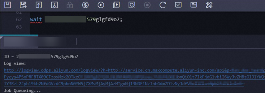
Run the following command to view job details:
DESC instance 2016070102275442go3xxxxxx;Response:
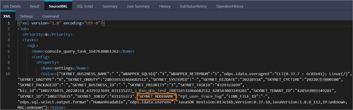
ID 2016070102275442go3xxxxxx
Owner ALIYUN$***@aliyun-inner.com
StartTime 2016-07-01 10:27:54
EndTime 2016-07-01 10:28:16
Status Terminated
console_query_task_1467340078684 Success
Query select count(*) from src where ds='20160628';
Open the LogView URL in your browser. In LogView, click the SourceXML tab to retrieve the SKYNET_NODENAME value.
 Note
NoteFor more information about LogView, see View job run information using Logview 2.0.
If the value of the SKYNET_NODENAME parameter cannot be retrieved or the SKYNET_NODENAME parameter has no value, you can obtain the code snippet from the SQL Script tab. You can then search for the code snippet in DataWorks to find and optimize the target node. For more information, see DataWorks code search.
In DataWorks, search for the node using the SKYNET_NODENAME value and optimize it.
Analyze job growth trends
Fees often increase due to job surges caused by repeated execution or misconfigured scheduling attributes.
Method 1: Analyze using Excel
Analyze records where Metering type is ComputationSql in the usage records. Count daily jobs per project and check for large fluctuations in job counts.
Method 2: Analyze using SQL
You have completed Step 2 and created the maxcomputefee table:
-- Analyze job growth trends.
SELECT  TO_CHAR(endtime,'yyyymmdd') AS ds
        ,projectid
        ,COUNT(*) AS tasknum
FROM    maxcomputefee
WHERE   TYPE = 'ComputationSql'
AND     TO_CHAR(endtime,'yyyymmdd') >= '20190112'
GROUP BY TO_CHAR(endtime,'yyyymmdd')
         ,projectid
ORDER BY tasknum DESC
LIMIT   10000
;
Observe job count trends for jobs submitted to and successfully run on MaxCompute between January 12 and January 14.
Analyze storage fees
Analyze why storage fees are CNY 0.01 using Excel:
After you activate the MaxCompute trial, no workloads run on MaxCompute, but you receive a ¥0.01 bill each day. This usually occurs because residual data is stored in MaxCompute, and the data volume does not exceed 0.5 GB.
Check records where Metering type is Storage. As shown in the figure, the
maxcompute_docproject stores 508 bytes. Per storage billing rules, data ≤ 512 MB incurs a fee of CNY 0.01.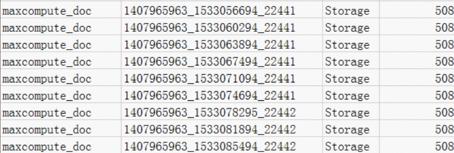 If this data is for testing only, resolve the issue as follows:
If only table data is unused, run the
Drop Tablestatement to delete table data in the project.If the project is unused, you can delete it in the MaxCompute console under .
Excel Analysis of
less than one daydata storage fees:Check records where Metering type is Storage. Assume the alian (example project name) project stores 333507833900 bytes. Because the data was uploaded at 08:00, billing starts at 09:07 and covers 15 hours.
Billing cycles end at the end of each day, so the last record is excluded from the April 4 bill.
Calculate the 24-hour average storage per storage billing rules, then apply the billing formula.
-- Calculate average storage.
333507833900 bytes × 15 / 1024 / 1024 / 1024 / 24 = 194.127109076362103 GB

-- Calculate daily storage fee, rounded to four decimal places.
194.127109076362103 GB × USD 0.0006 per GB per day = USD 0.1165 per day
Analyze storage fee distribution using SQL
You have completed Step 2 and created the maxcomputefee table:
-- Analyze storage fees.
SELECT  t.ds
        ,t.projectid
        ,t.storage
        ,CASE    WHEN t.storage < 0.5 THEN t.storage*0.01     -- Unit price is CNY 0.01 per GB per day if actual storage is > 0 MB and ≤ 512 MB.
                 WHEN t.storage >= 0.5  THEN t.storage*0.004  -- Unit price is CNY 0.004 per GB per day if actual storage is > 512 MB.
        END storage_fee
FROM    (
            SELECT  to_char(starttime,'yyyymmdd') as ds
                    ,projectid
                    ,SUM(storage/1024/1024/1024)/24 AS storage
            FROM    maxcomputefee
            WHERE   TYPE = 'Storage'
            and to_char(starttime,'yyyymmdd') >= '20190112'
            GROUP BY to_char(starttime,'yyyymmdd')
                     ,projectid
        ) t
ORDER BY storage_fee DESC
;
Results:
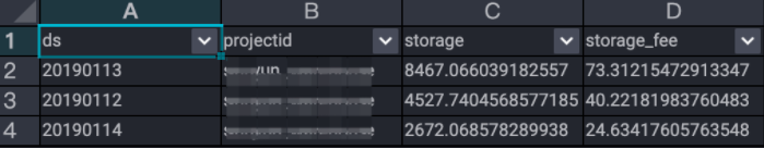 Conclusions:
Storage increased on January 12 and decreased on January 14.
To optimize storage, set lifecycles for tables and delete unnecessary temporary tables.
Analyze long-term storage, Infrequent Access (IA) storage, long-term storage access, and IA storage access using SQL
You have completed Step 2 and created the maxcomputefee table:
-- Analyze long-term storage fees.
SELECT  to_char(starttime,'yyyymmdd') as ds
        ,projectid
        ,SUM(storage/1024/1024/1024)/24*0.0011 AS longTerm_storage
  FROM  maxcomputefee
 WHERE  TYPE = 'ColdStorage'
   and  to_char(starttime,'yyyymmdd') >= '20190112'
GROUP BY to_char(starttime,'yyyymmdd')
         ,projectid;

-- Analyze IA storage fees.
SELECT  to_char(starttime,'yyyymmdd') as ds
        ,projectid
        ,SUM(storage/1024/1024/1024)/24*0.0011 AS lowFre_storage
  FROM  maxcomputefee
 WHERE  TYPE = 'LowFreqStorage'
   and  to_char(starttime,'yyyymmdd') >= '20190112'
GROUP BY to_char(starttime,'yyyymmdd')
         ,projectid;

-- Analyze long-term storage access fees.
SELECT  to_char(starttime,'yyyymmdd') as ds
        ,projectid
        ,SUM(computationsqlinput/1024/1024/1024)*0.522 AS longTerm_IO
  FROM  maxcomputefee
 WHERE  TYPE = 'SqlLongterm'
   and  to_char(starttime,'yyyymmdd') >= '20190112'
GROUP BY to_char(starttime,'yyyymmdd')
         ,projectid;

-- Analyze IA storage access fees.
SELECT  to_char(starttime,'yyyymmdd') as ds
        ,projectid
        ,SUM(computationsqlinput/1024/1024/1024)*0.522 AS lowFre_IO
  FROM  maxcomputefee
 WHERE  TYPE = 'SqlLowFrequency'
   and  to_char(starttime,'yyyymmdd') >= '20190112'
GROUP BY to_char(starttime,'yyyymmdd')
         ,projectid;
Analyze download fees
MaxCompute charges you for Internet-based or cross-region data downloads based on the amount downloaded.
Download fee = Downloaded data volume × Unit price (USD 0.1166 per GB)
Method 1: Analyze using Excel
Metering type = DownloadEx indicates Internet download billing.
For example, you find a record for download traffic of 0.036 GB (38,199,736 bytes). In this case, the download fee is calculated based on the billing rules that are described in Download pricing (pay-as-you-go) using the following formula:
(38,199,736 bytes/1024/1024/1024) × 0.1166 USD/GB = 0.004 USD.Optimize downloads. Check if your Tunnel service uses the public network, which incurs fees. For more information, see Endpoint. For bulk downloads, if you are in Suzhou and your region is China (Shanghai), first download data to a virtual machine using an ECS instance in China (Shanghai), then use your subscription ECS instance to download the data.
Method 2: Analyze using SQL
You have completed Step 2 and created the maxcomputefee table:
-- Analyze download fees.
SELECT  TO_CHAR(starttime,'yyyymmdd') AS ds
        ,projectid
        ,SUM((download/1024/1024/1024)*0.1166) AS download_fee
FROM    maxcomputefee
WHERE   type = 'DownloadEx'
AND     TO_CHAR(starttime,'yyyymmdd') >= '20190112'
GROUP BY TO_CHAR(starttime,'yyyymmdd')
         ,projectid
ORDER BY download_fee DESC
;
Analyze MapReduce Job Consumption
MapReduce job fee = Total billable hours × Unit price (USD 0.0690 per hour per task)
Method 1: Analyze using Excel
Analyze records where Metering type is MapReduce in the usage records. Calculate and sort MapReduce job fees by specification type. MapReduce job fee formula:
(MR/Spark compute (core*second)/3600 × Unit price (USD 0.0690))Method 2: Analyze using SQL
You have completed Step 2 and created the maxcomputefee table:
-- Analyze MapReduce job fees.
SELECT  TO_CHAR(starttime,'yyyymmdd') AS ds
        ,projectid
        ,(cu_usage/3600)*0.0690 AS mr_fee
FROM    maxcomputefee
WHERE   type = 'MapReduce'
AND     TO_CHAR(starttime,'yyyymmdd') >= '20190112'
GROUP BY TO_CHAR(starttime,'yyyymmdd')
         ,projectid
         ,cu_usage
ORDER BY mr_fee DESC
;
Analyze external table jobs (Tablestore and OSS)
SQL external table fee = Input data volume × Unit price (USD 0.0044 per GB)
Method 1: Analyze using Excel
Analyze records where Metering type is ComputationSqlOTS or ComputationSqlOSS in the usage records. Sort SQL external table fees. Fee formula:
SQL input (bytes)/1024/1024/1024 × Unit price (USD 0.0044).Method 2: Analyze using SQL
You have completed Step 2 and created the maxcomputefee table:
-- Analyze Tablestore external table SQL job fees.
SELECT  TO_CHAR(starttime,'yyyymmdd') AS ds
        ,projectid
        ,(computationsqlinput/1024/1024/1024)*1*0.03 AS ots_fee
FROM    maxcomputefee
WHERE   type = 'ComputationSqlOTS'
AND     TO_CHAR(starttime,'yyyymmdd') >= '20190112'
GROUP BY TO_CHAR(starttime,'yyyymmdd')
         ,projectid
         ,computationsqlinput
ORDER BY ots_fee DESC
;

-- Analyze OSS external table SQL job fees.
SELECT  TO_CHAR(starttime,'yyyymmdd') AS ds
        ,projectid
        ,(computationsqlinput/1024/1024/1024)*1*0.03 AS oss_fee
FROM    maxcomputefee
WHERE   type = 'ComputationSqlOSS'
AND     TO_CHAR(starttime,'yyyymmdd') >= '20190112'
GROUP BY TO_CHAR(starttime,'yyyymmdd')
         ,projectid
         ,computationsqlinput
ORDER BY oss_fee DESC
;
Analyze Spark compute fees
Spark job fee = Total billable hours × Unit price (USD 0.1041 per hour per task)
Method 1: Analyze using Excel
Analyze records where Metering type is Spark in the usage records. Sort job fees. Fee formula:
(MR/Spark compute (core*second)/3600 × Unit price (USD 0.1041)).Method 2: Analyze using SQL
You have completed Step 2 and created the maxcomputefee table:
-- Analyze Spark job fees.
SELECT  TO_CHAR(starttime,'yyyymmdd') AS ds
        ,projectid
        ,(cu_usage/3600)*0.1041 AS mr_fee
FROM    maxcomputefee
WHERE   type = 'spark'
AND     TO_CHAR(starttime,'yyyymmdd') >= '20190112'
GROUP BY TO_CHAR(starttime,'yyyymmdd')
         ,projectid
         ,cu_usage
ORDER BY mr_fee DESC
;