The aliyun-timestream plug-in, developed by the Alibaba Cloud Elasticsearch team, lets you manage time series indexes through a dedicated API—without writing complex domain-specific language (DSL) queries. Use PromQL to query metric data stored in your cluster, and benefit from built-in Elasticsearch best practices for time series storage to reduce disk usage.
For a full overview of the plug-in, see Overview of aliyun-timestream. For the complete API reference and Prometheus integration, see Overview of APIs supported by aliyun-timestream and Integrate aliyun-timestream with Prometheus APIs.
When to use aliyun-timestream
Use the aliyun-timestream plug-in when your data meets all of the following criteria:
-
Data consists of metric measurements with timestamps (CPU usage, memory, disk I/O, and similar)
-
Data is written in near real-time and roughly in
@timestamporder -
Each data point is identified by a set of dimension fields (labels such as
clusterId,nodeId,namespace) -
You plan to query data using PromQL or Elasticsearch aggregations
A time series index created through aliyun-timestream is built on top of Elasticsearch's data stream, with automatic configuration of index.mode: time_series, the aliyun-codec compression plug-in, and dimension-based routing. This differs from a regular index or data stream in several key ways:
-
Time-bound backing indexes: Data from the same time window is routed to the same backing index, based on
index.time_series.start_timeandindex.time_series.end_time. -
Dimension-based routing: All data points sharing the same dimension values are stored on the same shard, identified by an internal
_tsidfield. This improves compression and query performance. -
Metric field storage: Metric fields store only doc values and do not store inverted index data, which reduces disk usage.
-
PromQL support: Query metric data using PromQL through the plug-in's Prometheus-compatible API, rather than DSL.
Prerequisites
Before you begin, ensure that you have:
-
An Alibaba Cloud Elasticsearch cluster of Standard Edition meeting one of the following version requirements:
-
Cluster version V7.16 or later, and kernel version V1.7.0 or later
-
Cluster version V7.10, and kernel version V1.8.0 or later
-
For instructions on creating a cluster, see Create an Alibaba Cloud Elasticsearch cluster.
Manage time series indexes
Create a time series index
Create a time series index named test_stream:
PUT _time_stream/test_streamThis creates an Elasticsearch data stream (not a standalone index), along with an index template named .timestream_test_stream that pre-configures the following settings:
| Setting | Value | Effect |
|---|---|---|
index.mode |
time_series |
Enables time series mode with built-in Elasticsearch best practices for time series storage |
index.codec |
ali |
Activates the aliyun-codec index compression plug-in |
index.ali_codec_service.enabled |
true |
Enables index compression |
index.doc_value.compression.default |
zstd |
Compresses column-oriented (doc values) data using the zstd algorithm |
index.postings.compression |
zstd |
Compresses inverted index data using zstd |
index.ali_codec_service.source_reuse_doc_values.enabled |
true |
Enables source reuse from doc values to reduce storage |
index.source.compression |
zstd |
Compresses row-oriented (source) data using zstd |
index.translog.durability |
ASYNC |
Reduces write latency by using asynchronous translog writes |
index.refresh_interval |
10s |
Batches index refreshes to improve write throughput |
index.routing_path |
labels.* |
Routes documents to shards based on label fields |
The index template also pre-configures mappings for two field categories:
-
Dimension fields (
labels.*): Mapped askeywordwithtime_series_dimension: true. All dimension fields are combined into the internal_tsidfield, which uniquely identifies each time series. -
Metric fields (
metrics.*): Mapped asdoubleorlongwith"index": false. Only doc values are stored—no inverted index data.
View the full configuration of test_stream:
GET _time_stream/test_streamCustomize the index template
Pass a template body when creating the index to override default settings. The following examples show common customizations:
-
Set the number of primary shards:
PUT _time_stream/test_stream { "template": { "settings": { "index": { "number_of_shards": "2" } } } } -
Customize the data model (field naming conventions):
PUT _time_stream/test_stream
{
  "template": {
    "settings": {
      "index": {
        "number_of_shards": "2"
      }
    }
  },
  "time_stream": {
    "labels_fields": ["labels_*"],
    "metrics_fields": ["metrics_*"]
  }
}
Update a time series index
Update the number of primary shards for test_stream:
POST _time_stream/test_stream/_update
{
  "template": {
    "settings": {
      "index": {
        "number_of_shards": "4"
      }
    }
  }
}Include all existing configurations in the update request body, not just the fields you want to change. Omitting a field resets it to its default. Run GET _time_stream/test_stream first to retrieve the full current configuration, then modify the fields you need.
After updating, the new settings do not apply to the current backing index. Roll over the index to apply them:
POST test_stream/_rolloverA new backing index is created with the updated settings. The original backing index retains its previous settings.
Delete a time series index
Delete test_stream and all its data:
DELETE _time_stream/test_streamThis deletes all data in the index and its configuration. This operation cannot be undone.
Write and query time series data
Time series indexes are used in the same way as regular Elasticsearch indexes for data writes and basic queries.
Write data
Use the bulk or index API to write documents. Each document must include an @timestamp field set to the time the measurement was taken.
POST test_stream/_doc
{
  "@timestamp": 1630465208722,
  "metrics": {
    "cpu.idle": 79.67298116109929,
    "disk_ioutil": 17.630910821570456,
    "mem.free": 75.79973639970004
  },
  "labels": {
    "disk_type": "disk_type2",
    "namespace": "namespaces1",
    "clusterId": "clusterId3",
    "nodeId": "nodeId5"
  }
}
How time-based routing works
Each backing index in the data stream has a time range defined by index.time_series.start_time and index.time_series.end_time. A document is written to the backing index whose time range contains the document's @timestamp value.
The data stream manages this time range automatically. After a rollover, the new backing index takes over from the end time of the previous index, so all backing indexes together cover a continuous time range with no gaps.
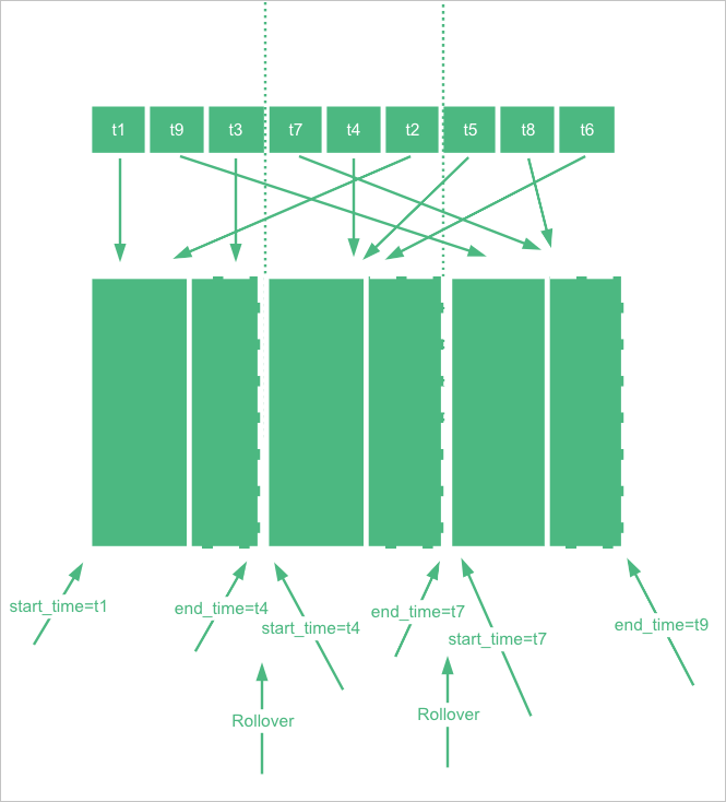
Time range boundaries are in UTC. If your application runs in UTC+8, convert accordingly: for example, 2022-06-21T00:00:00.000Z (UTC) corresponds to 2022-06-21T08:00:00.000 in UTC+8.
Query data
Search all documents in test_stream:
GET test_stream/_searchView index details:
GET _cat/indices/test_stream?v&s=iView index statistics
Get statistics for test_stream, including the number of time series tracked per shard:
GET _time_stream/test_stream/_statsExample response:
{
  "_shards" : {
    "total" : 2,
    "successful" : 2,
    "failed" : 0
  },
  "time_stream_count" : 1,
  "indices_count" : 1,
  "total_store_size_bytes" : 19132,
  "time_streams" : [
    {
      "time_stream" : "test_stream",
      "indices_count" : 1,
      "store_size_bytes" : 19132,
      "tsid_count" : 2
    }
  ]
}
The time_stream_count metric counts unique time series per primary shard by reading the _tsid field's doc values. This is a relatively expensive operation. To reduce the cost:
-
For read-only indexes, configure a caching policy so that the count is collected only once and not refreshed again.
-
For active indexes, the cache refreshes every 5 minutes by default. Adjust this interval with the
index.time_series.stats.refresh_intervalparameter. The minimum value is 1 minute.
Use Prometheus APIs to query data
The aliyun-timestream plug-in exposes a Prometheus-compatible query interface at /_time_stream/prom/{index_name}. Use this to integrate with Grafana or any Prometheus-compatible tool.
Configure a Prometheus data source
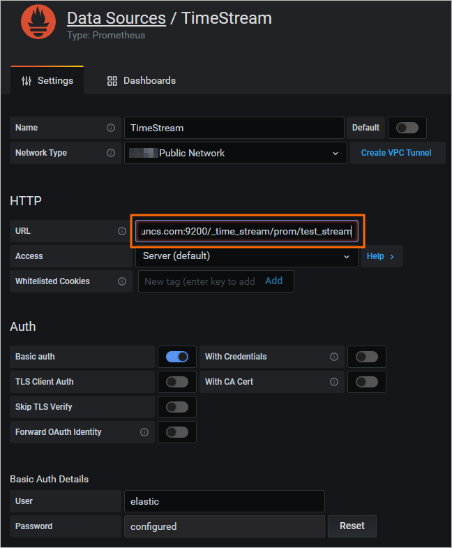
Option 1: Grafana console
In the Grafana console, add a Prometheus data source and set the URL to /_time_stream/prom/test_stream. The time series index is then available as a Prometheus data source directly.
Option 2: Custom field prefixes and suffixes
When querying through the Prometheus API, the plug-in strips the metrics. prefix from metric fields and the labels. prefix from dimension fields by default.
If you created the index with a custom data model (non-default field prefixes), configure the prefix and suffix mappings explicitly:
PUT _time_stream/{name}
{
  "time_stream": {
    "labels_fields": "@labels.*_l",
    "metrics_fields": "@metrics.*_m",
    "label_prefix": "@labels.",
    "label_suffix": "_l",
    "metric_prefix": "@metrics.",
    "metric_suffix": "_m"
  }
}
Query metadata
View all metric fields in test_stream:
GET /_time_stream/prom/test_stream/metadataExample response:
{
  "status" : "success",
  "data" : {
    "cpu.idle" : [
      {
        "type" : "gauge",
        "help" : "",
        "unit" : ""
      }
    ],
    "disk_ioutil" : [
      {
        "type" : "gauge",
        "help" : "",
        "unit" : ""
      }
    ],
    "mem.free" : [
      {
        "type" : "gauge",
        "help" : "",
        "unit" : ""
      }
    ]
  }
}
View all dimension fields in test_stream:
GET /_time_stream/prom/test_stream/labelsExample response:
{
  "status" : "success",
  "data" : [
    "__name__",
    "clusterId",
    "disk_type",
    "namespace",
    "nodeId"
  ]
}
View all values for a specific dimension field:
GET /_time_stream/prom/test_stream/label/clusterId/valuesExample response:
{
  "status" : "success",
  "data" : [
    "clusterId1",
    "clusterId3"
  ]
}
View all time series for the cpu.idle metric:
GET /_time_stream/prom/test_stream/series?match[]=cpu.idleExample response:
{
  "status" : "success",
  "data" : [
    {
      "__name__" : "cpu.idle",
      "disk_type" : "disk_type1",
      "namespace" : "namespaces2",
      "clusterId" : "clusterId1",
      "nodeId" : "nodeId2"
    },
    {
      "__name__" : "cpu.idle",
      "disk_type" : "disk_type1",
      "namespace" : "namespaces2",
      "clusterId" : "clusterId1",
      "nodeId" : "nodeId5"
    },
    {
      "__name__" : "cpu.idle",
      "disk_type" : "disk_type2",
      "namespace" : "namespaces1",
      "clusterId" : "clusterId3",
      "nodeId" : "nodeId5"
    }
  ]
}
Query data with PromQL
Use the Prometheus instant query and range query APIs to run PromQL queries against your time series index. For details on supported PromQL syntax, see Support of aliyun-timestream for PromQL.
Instant query
GET /_time_stream/prom/test_stream/query?query=cpu.idle&time=1655769837The time parameter is in Unix seconds. If omitted, the query returns data from the previous 5 minutes.
Example response:
{
  "status" : "success",
  "data" : {
    "resultType" : "vector",
    "result" : [
      {
        "metric" : {
          "__name__" : "cpu.idle",
          "clusterId" : "clusterId1",
          "disk_type" : "disk_type1",
          "namespace" : "namespaces2",
          "nodeId" : "nodeId2"
        },
        "value" : [
          1655769837,
          "79.672981161"
        ]
      },
      {
        "metric" : {
          "__name__" : "cpu.idle",
          "clusterId" : "clusterId1",
          "disk_type" : "disk_type1",
          "namespace" : "namespaces2",
          "nodeId" : "nodeId5"
        },
        "value" : [
          1655769837,
          "79.672981161"
        ]
      },
      {
        "metric" : {
          "__name__" : "cpu.idle",
          "clusterId" : "clusterId3",
          "disk_type" : "disk_type2",
          "namespace" : "namespaces1",
          "nodeId" : "nodeId5"
        },
        "value" : [
          1655769837,
          "79.672981161"
        ]
      }
    ]
  }
}
Range query
GET /_time_stream/prom/test_stream/query_range?query=cpu.idle&start=1655769800&end=16557699860&step=1mExample response:
{
  "status" : "success",
  "data" : {
    "resultType" : "matrix",
    "result" : [
      {
        "metric" : {
          "__name__" : "cpu.idle",
          "clusterId" : "clusterId1",
          "disk_type" : "disk_type1",
          "namespace" : "namespaces2",
          "nodeId" : "nodeId2"
        },
        "value" : [
          [
            1655769860,
            "79.672981161"
          ]
        ]
      },
      {
        "metric" : {
          "__name__" : "cpu.idle",
          "clusterId" : "clusterId1",
          "disk_type" : "disk_type1",
          "namespace" : "namespaces2",
          "nodeId" : "nodeId5"
        },
        "value" : [
          [
            1655769860,
            "79.672981161"
          ]
        ]
      },
      {
        "metric" : {
          "__name__" : "cpu.idle",
          "clusterId" : "clusterId3",
          "disk_type" : "disk_type2",
          "namespace" : "namespaces1",
          "nodeId" : "nodeId5"
        },
        "value" : [
          [
            1655769860,
            "79.672981161"
          ]
        ]
      }
    ]
  }
}
Configure downsampling
Downsampling reduces the resolution of older time series data to speed up queries over large time ranges. The plug-in automatically selects the most appropriate downsampling index based on the fixed_interval value in your aggregation query.
Configure downsampling intervals when creating a time series index. The following example configures three downsampling intervals: 1 minute, 10 minutes, and 60 minutes.
PUT _time_stream/test_stream
{
  "time_stream": {
    "downsample": [
      {
        "interval": "1m"
      },
      {
        "interval": "10m"
      },
      {
        "interval": "60m"
      }
    ]
  }
}
After data is written and the original backing index is rolled over, the plug-in automatically generates downsampling indexes from the original backing index. Downsampling starts when the current time is at least two hours past the index's end_time.
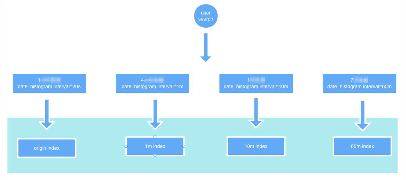
How automatic index selection works
When you run an aggregation query, pass the original index name and specify fixed_interval in the date_histogram aggregation. The plug-in selects the downsampling index with the highest time precision that is still a multiple of fixed_interval.
For example, if fixed_interval is 120m and downsampling intervals are 1m, 10m, and 60m, the plug-in queries the 60m downsampling index.
Example query using fixed_interval: 120m:
GET test_stream/_search?size=0&request_cache=false
{
  "aggs": {
    "1": {
      "terms": {
        "field": "labels.disk_type",
        "size": 10
      },
      "aggs": {
        "2": {
          "date_histogram": {
            "field": "@timestamp",
            "fixed_interval": "120m"
          }
        }
      }
    }
  }
}
Example response (querying the 60m downsampling index):
{
  "took" : 15,
  "timed_out" : false,
  "_shards" : {
    "total" : 2,
    "successful" : 2,
    "skipped" : 0,
    "failed" : 0
  },
  "hits" : {
    "total" : {
      "value" : 1,
      "relation" : "eq"
    },
    "max_score" : null,
    "hits" : [ ]
  },
  "aggregations" : {
    "1" : {
      "doc_count_error_upper_bound" : 0,
      "sum_other_doc_count" : 0,
      "buckets" : [
        {
          "key" : "disk_type2",
          "doc_count" : 9,
          "2" : {
            "buckets" : [
              {
                "key_as_string" : "2022-06-20T06:00:00.000Z",
                "key" : 1655704800000,
                "doc_count" : 9
              }
            ]
          }
        }
      ]
    }
  }
}
hits.total.value is 1, meaning one downsampled record was returned. The doc_count of 9 in the aggregations indicates that 9 original data points were rolled up into that record, confirming the query hit the downsampling index rather than the original.
For comparison, setting fixed_interval to 20s queries the original index and returns hits.total.value: 9, matching doc_count: 9.
Downsampling indexes have the same settings and mappings as the original index, except that data is aggregated into time buckets based on the configured interval.
Test downsampling with a demo index
The following procedure demonstrates the full downsampling lifecycle using a manually controlled time range. This is useful for testing and validation. In production, the plug-in triggers downsampling automatically after rollover.
-
Create an index with a fixed time range and downsampling configuration. The
start_timeandend_timevalues simulate a past time window so the downsampling trigger condition (current time is at least two hours pastend_time) is immediately satisfied.ImportantAfter this step, check
end_timeby runningGET {index}/_settings. The system adjustsend_timeevery 5 minutes by default. Proceed to the next step beforeend_timeis updated.PUT _time_stream/test_stream { "template": { "settings": { "index.time_series.start_time": "2022-06-20T00:00:00.000Z", "index.time_series.end_time": "2022-06-21T00:00:00.000Z" } }, "time_stream": { "downsample": [ { "interval": "1m" }, { "interval": "10m" }, { "interval": "60m" } ] } } -
Write a document with
@timestampset to a value within the[start_time, end_time)range:POST test_stream/_doc { "@timestamp": 1655706106000, "metrics": { "cpu.idle": 79.67298116109929, "disk_ioutil": 17.630910821570456, "mem.free": 75.79973639970004 }, "labels": { "disk_type": "disk_type2", "namespace": "namespaces1", "clusterId": "clusterId3", "nodeId": "nodeId5" } } -
Remove
start_timeandend_timefrom the index, and keep the downsampling configuration:POST _time_stream/test_stream/_update { "time_stream": { "downsample": [ { "interval": "1m" }, { "interval": "10m" }, { "interval": "60m" } ] } } -
Roll over the index:
POST test_stream/_rollover -
After the rollover completes, view the generated downsampling indexes:
GET _cat/indices/test_stream?v&s=iExpected output:
health status index                                          uuid                   pri rep docs.count docs.deleted store.size pri.store.size
green  open   .ds-test_stream-2022.06.21-000001              vhEwKIlwSGO3ax4RKn****   1   1          9            0     18.5kb         12.1kb
green  open   .ds-test_stream-2022.06.21-000001_interval_10m r9Tsj0v-SyWJDc64oC****   1   1          1            0     15.8kb          7.9kb
green  open   .ds-test_stream-2022.06.21-000001_interval_1h  cKsAlMK-T2-luefNAF****   1   1          1            0     15.8kb          7.9kb
green  open   .ds-test_stream-2022.06.21-000001_interval_1m  L6ocasDFTz-c89KjND****   1   1          1            0     15.8kb          7.9kb
green  open   .ds-test_stream-2022.06.21-000002              42vlHEFFQrmMAdNdCz****   1   1          0            0       452b           226b
The three downsampling indexes (
_interval_1m,_interval_10m,_interval_1h) are created alongside the new backing index (000002).
What's next
-
Overview of APIs supported by aliyun-timestream — full API reference including downsampling API usage notes
-
Integrate aliyun-timestream with Prometheus APIs — complete Prometheus API integration guide and PromQL support details