Analyze data with an online spreadsheet
When you need to perform quick, ad hoc analysis on small datasets or use a flexible, Excel-like tool to organize, calculate, and visualize data, traditional SQL queries can be cumbersome and professional BI tools often have a steep learning curve. DataWorks Data Analysis offers a spreadsheet feature: an online, Excel-like tool where you can enter and edit data or import local files, just as you would in a local spreadsheet.
Edition limits
Chart type limit: The Basic Edition supports only seven chart types. To access more chart types, upgrade to DataWorks Standard Edition or higher.
Spreadsheet sharing limits: The maximum number of editors and viewers varies by edition.
Feature
Basic Edition
Standard Edition
Professional Edition
Enterprise Edition
Maximum number of editors
0
3
5
10
Maximum number of viewers
0
10
20
30
Access spreadsheets
From the Data Analysis page, click Go to Data Analysis. On the left menu bar, click the ![]() or
or ![]() icon to go to the Spreadsheet list page.
icon to go to the Spreadsheet list page.
Create a spreadsheet
Before you can analyze data, you need to create a spreadsheet.
New data analysis
On the Spreadsheet page, in the upper-right corner of the directory tree on the left, click the

In the spreadsheet editor, after you finish your data analysis, click Save in the upper-right corner.
In the Save File dialog box, enter a File Name and click OK.
Legacy data analysis
On the Spreadsheet page, click the
 icon under New Spreadsheet to open the spreadsheet editor.
In the spreadsheet editor, after you finish your data analysis, click Save in the upper-right corner.
In the Save File dialog box, enter a File Name and click OK.
Import data to a spreadsheet
You can enter data directly into a spreadsheet or import it from local files for analysis.
On the spreadsheet editing page, click Import in the upper-right corner. You can import data from a Spreadsheet, a Local CSV File, or a Local Excel File.
Import a spreadsheet
In the Import dialog box, click Spreadsheet and configure the following parameters.
Parameter | Description |
Spreadsheet | From the Spreadsheet drop-down list, select the spreadsheet to import. |
Sheet | From the Sheet drop-down list, select the sheet to import from the spreadsheet. |
Data preview | Previews the data to be imported. |
Import Start Row | Specifies the starting row for the import. The default value is 1. |
Placement Location | The available options are Current Worksheet and New Worksheet. |
Placement Method | The available options are Append, Overwrite, and Active Cell. |
Import a local CSV file
In the Import dialog box, click Local CSV File and configure the following parameters.
Parameter | Description |
File | Click Choose file, select the local CSV file to import, and then click Open. |
Original Character Set | The available options are UTF-8 and GBK. If garbled characters appear, try switching the character set. |
Separator | Specifies the row and column separators.
If the data is not separated correctly into cells, try switching the separator. |
Data preview | Previews the data to be imported. |
Import Start Row | Specifies the starting row for the import. The default value is 1. |
Placement Location | Current Worksheet: Imports the data into the currently active worksheet. New Worksheet: Creates a new worksheet and imports the data into it. |
Placement Method | The available options are Append, Overwrite, and Active Cell. |
Import a local Excel file
In the Import dialog box, click Local Excel File and configure the following parameters.
Parameter | Description |
File | Click Choose file, select the local Excel file to import, and then click Open. |
Sheet | From the Sheet drop-down list, select the sheet to import. |
Data preview | Previews the data to be imported. |
Import Start Row | Specifies the starting row for the import. The default value is 1. |
Placement Location | The available options are Current Worksheet and New Worksheet. |
Placement Method | The available options are Append, Overwrite, and Active Cell. |
Analyze data
The spreadsheet provides a range of data analysis features similar to Microsoft Excel. On the spreadsheet editing page, you can customize the font, alignment, number format, rows and columns, conditional formatting, and styles. You can also explore your data.
For a detailed description of each button in the spreadsheet, see Appendix: Detailed description of each button.
Formatting and styles

In the top toolbar, adjust the font, alignment, number format (such as currency and percentage), and conditional formatting of cells to improve readability.
Formulas and functions

Just like in Excel, enter = in a cell to start a formula. The spreadsheet supports common functions such as SUM and AVERAGE.
Charts

Select the data range to analyze.
In the top menu bar, choose Chart and select a chart type, such as a bar chart, line chart, or pie chart.
The system automatically identifies the data types and generates a chart.
ImportantIf the chart does not look as expected, try right-clicking the target column and selecting Convert to Numeric.
Data profiling
The data profiling feature analyzes your data's quality, structure, distribution, and statistics, allowing you to preview, explore, process, analyze, and visualize it.
Simple data profiling mode: Select your data and click Data Profiling in the top toolbar. The system automatically analyzes each column's type, distribution, null value, and duplicate value, giving you a quick overview of your data quality.
Detailed data profiling mode: In simple profiling mode, click Detailed Mode in the upper-right corner to view profiling results for each column, including Field Name, Field Type, Field Chinese Name, Field Description, and Security Level.

Type | Simple mode | Detailed mode |
String / Date | Displays information in a rich text format: | Displays detailed information, including: |
Integer / Float | Displays a binned histogram to visualize the data's range and distribution. | Displays detailed information, including: |
Boolean | Displays a pie chart to show the percentage of true and false values. | Displays detailed information, including: String values of true and false, and numeric values of 0 and 1, are treated as the boolean type. |
mixed type | Displays a pie chart showing the percentage of each data type in the column and indicates the presence of dirty data. Once cleaned, the value distribution is displayed according to one of the three preceding types. | Not applicable (in detailed mode, the system analyzes each field based on its predefined type). |
Null | The percentage of | This appears as the null rate in the basic information for each type. |
Manage spreadsheets
On the spreadsheet editing page, click Spreadsheet in the upper-left corner or the
 icon in the left menu bar to open the spreadsheet list.
On the Spreadsheet page, in the All Spreadsheets section, you can view spreadsheets in the I created and Share it with me lists.
On the list page, you can manage spreadsheets as follows:
Rename: Click the
icon next to the file. In the Rename dialog box, enter a new File Name and click OK.Change owner: Click the
icon next to the file. In the Change Owner dialog box, enter and select the new owner, then click OK.Clone: Click the
icon next to the file. This creates a new file with the suffix _copy.Delete: Click the
icon next to the file. In the Delete dialog box, click OK.
Click a File Name to return to the spreadsheet editing page.
Export, share, and download a spreadsheet
After you process and analyze data in an online spreadsheet, you can export, download, or share the data with specific users.

Export data to MaxCompute
You can use a spreadsheet to quickly generate a MaxCompute CREATE TABLE statement based on the processed data. After you copy the statement, go to DataStudio to export the data to a MaxCompute table. You can export a maximum of 100 rows of data.
On the spreadsheet editing page, click in the upper-right corner.
In the Export as MaxCompute Table dialog box, configure the parameters.
Insert mode
Parameter
Description
Insert data into a MaxCompute table (insert overwrite)
Workspace
Select the target project.
Table
Enter the name of the table and select it.
Create MaxCompute Table and Insert Data (INSERT OVERWRITE)
Workspace
Select the target project.
Table Name
Enter a name for the new table and click Check Duplicate Names to verify its uniqueness.
Click Copy SQL Statement and then click Close.
ImportantOnly non-partitioned tables are supported. You can copy a maximum of 100 rows of data.
In the upper-left corner of the page, click the
icon and select All Products > Data Development and O&M > DataStudio (Data Development).Use a MaxCompute SQL node to insert data into an existing table or to create and populate a new MaxCompute table.
For operations in the new version of DataStudio, see Develop a MaxCompute SQL node.
For operations in the old version of DataStudio, see Develop an ODPS SQL task.
Click Submit to Development Environment and Submit to Production Environment.
If you are using a workspace in basic mode, you only need to click Submit to Production.

Share a spreadsheet
Common scenarios for sharing a spreadsheet include:
Multi-user collaboration: Share the spreadsheet and grant edit permissions to other users. For example, you can use this feature to collect personal information from team members or manage event registrations.
Read-only sharing: Share the spreadsheet and grant read permissions to other users.
If you see a permission error, contact your tenant administrator. The administrator must navigate to Security Center > Data Query and Control > Query result control and enable Allow Sharing and Allow Download for Spreadsheet. For more information, see Data Query and Analysis Control.
On the spreadsheet editing page, click Share in the upper-right corner to configure the sharing settings.
Link: After you specify members with edit or read permissions, or make the spreadsheet visible to everyone, click Copy Link and send the link to the intended users.
If you enable Access Code, a link is generated that requires an access code.
Specify Editable Members: To grant specific users permission to edit the spreadsheet, click Specify Editable Members > Add. In the dialog box, enter and select the members, and then click Confirm.
Visible to All: To make the spreadsheet accessible to everyone, turn on the Visible to All toggle.
The following members can view: To grant specific users permission to read the spreadsheet, turn off Visible to All and then click The following members can view > Add. In the dialog box, enter and select the members, and then click Confirm.

After you share the spreadsheet, send the link to the recipients so they can access it.
On the spreadsheet editing page, click View Records in the upper-right corner to see who has viewed the shared spreadsheet.
On the Spreadsheet list, you can find spreadsheets shared with you under Share it with me.
Download a spreadsheet
On the spreadsheet editing page, click Download in the upper-right corner to save the spreadsheet to your computer.
Appendix: Buttons and features
In the spreadsheet editor, you can configure the following settings:
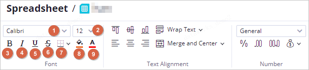
Font
No.
Feature
Description
①
Font
Sets the font for the text.
②
Font size
Sets the font size.
③
Bold
Makes the text bold.
④
Italic
Italicizes the text.
⑤
Underline
Underlines the text.
⑥
Strikethrough
Applies a strikethrough to the text.
⑦
Borders
Adds borders to cells.
⑧
Fill color
Changes the background color of cells.
⑨
Font color
Changes the color of the text.
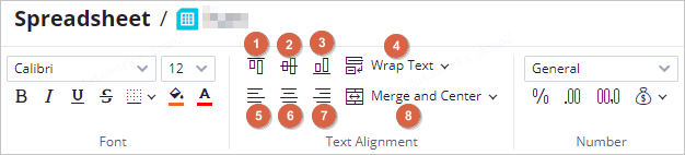
Text Alignment
No.
Feature
Description
①
Top Align
Aligns text to the top of the cell.
②
Middle Align
Centers text vertically within the cell.
③
Bottom Align
Aligns text to the bottom of the cell.
④
Wrap Text
Wraps lengthy text onto multiple lines to fit the cell width.
⑤
Align Left
Aligns text to the left.
⑥
Center
Centers text horizontally.
⑦
Align Right
Aligns text to the right.
⑧
Merge and Center
Merges selected cells into a single cell and centers the content.
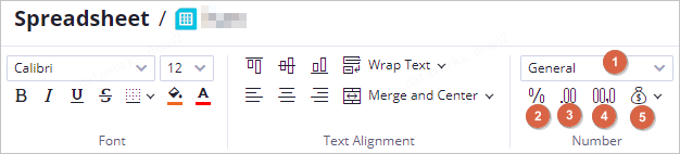
Number
No.
Feature
Description
①
Data type
Sets the data type for cells, with options such as number, currency, date, time, and text.
②
Percentage
Formats the selected cells as a percentage.
③
Two Decimal Places
Formats the number to two decimal places.
④
1000 Separator
Formats the number with a thousand separator, for example, 1,005.
⑤
Currency
Formats the selected cells as a currency, such as yuan, US dollar, pound sterling, euro, and franc.
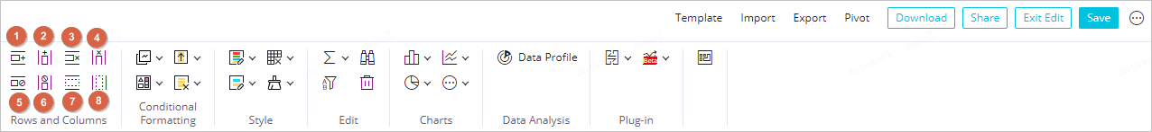
Rows and Columns
No.
Feature
Description
①
Insert Row
Adds a new row to the sheet.
②
Insert column
Adds a new column to the sheet.
③
Delete Row
Deletes the selected row.
④
Delete column
Deletes the selected column.
⑤
Lock Row
Keeps all rows above the selection visible while you scroll.
⑥
Lock Column
Keeps all columns to the left of the selection visible while you scroll.
⑦
Hide Row
Hides the selected row.
⑧
Hide Column
Hides the selected column.
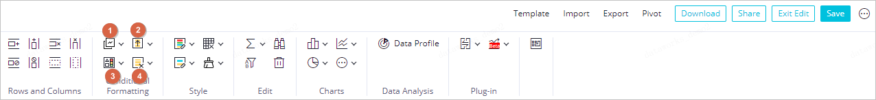
Conditional Formatting
No.
Feature
Description
①
Filter-based conditional formatting
Includes highlight cells rules and Top/Bottom Rules.
②
Color fill conditional formatting
Includes Gradient Fill, Solid Fill, and Color Scales.
③
Icon set conditional formatting
Includes Directional, Shapes, Indicators, and Ratings icons.
④
Clear conditional formatting
Includes options to Clear Rules from Selected Cells and Clear Rules from Entire Sheet.
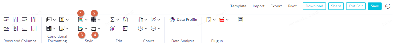
Style
No.
Feature
Description
①
Apply table style
Applies a pre-defined style to a table.
②
Delete
Removes the applied table style.
③
Cell Style
Applies a style to the selected cells.
④
Clear
Includes options to Clear All, Clear Content, and Clear Style.
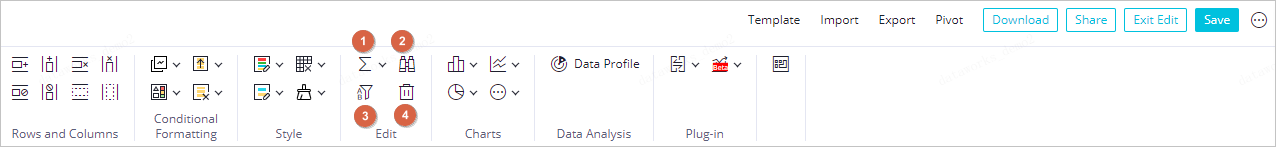
Edit
No.
Feature
Description
①
AutoSum
Provides quick access to five common functions: Sum, Average, Count Numbers, max, and min.
②
Search
Click Search or press Ctrl+F to open the search box.
③
Sort and Filter
Filters data and sorts it in ascending or descending order.
④
Clear
Deletes the content of the selected cells.
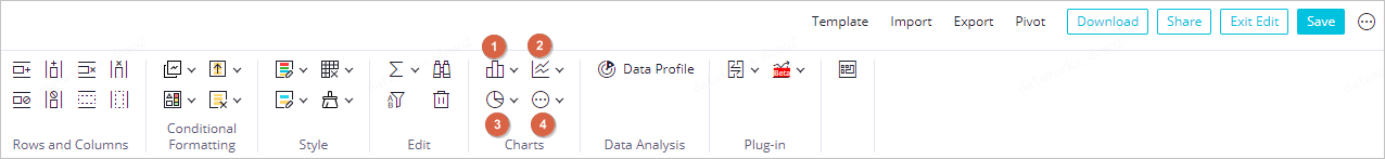
Charts
No.
Feature
Description
①
Column Chart
For details, see Column Chart.
②
Line Chart
For details, see Line Chart.
③
Pie chart
For details, see Pie Chart.
④
More
Click More to select from the following chart types:
Stock Chart
Plug-in: Currently supports Type Conversion. Click the
icon to apply Convert to Numeric or Convert to String to selected data.List of Shortcut Keys: Click the
icon to view a list of available shortcut keys.