How ARMS calculates quantile metrics
Application Real-Time Monitoring Service (ARMS) uses quantile metrics such as P50, P75, P90, and P99 to represent latency distributions across your application. This topic covers how the ARMS agent computes these quantiles, the accuracy trade-offs of the histogram approach, and when to use agent-based quantiles versus Trace Explorer quantiles.
Quantile metrics in monitoring
Average latency hides outliers. If 99% of requests complete in 10 ms but 1% take 5,000 ms, the average looks healthy while a significant portion of users experience poor performance.
Quantiles (also called percentiles) solve this by showing the latency at specific points in the distribution:
| Quantile | Meaning |
|---|---|
| P50 | The median. Half of all requests are faster, half are slower. |
| P75 | 75% of requests complete at or below this latency. |
| P90 | 90% of requests complete at or below this latency. |
| P99 | 99% of requests complete at or below this latency. Only 1% are slower. |
P90 and P99 are especially useful for understanding tail latency -- the experience of your slowest users.
Example
Given 14 data points: [2, 3, 6, 7, 8, 9, 10, 12, 14, 15, 16, 17, 18, 20]
The exact quantile values are:
P50: 10
P75: 16
P90: 18
P99: 20
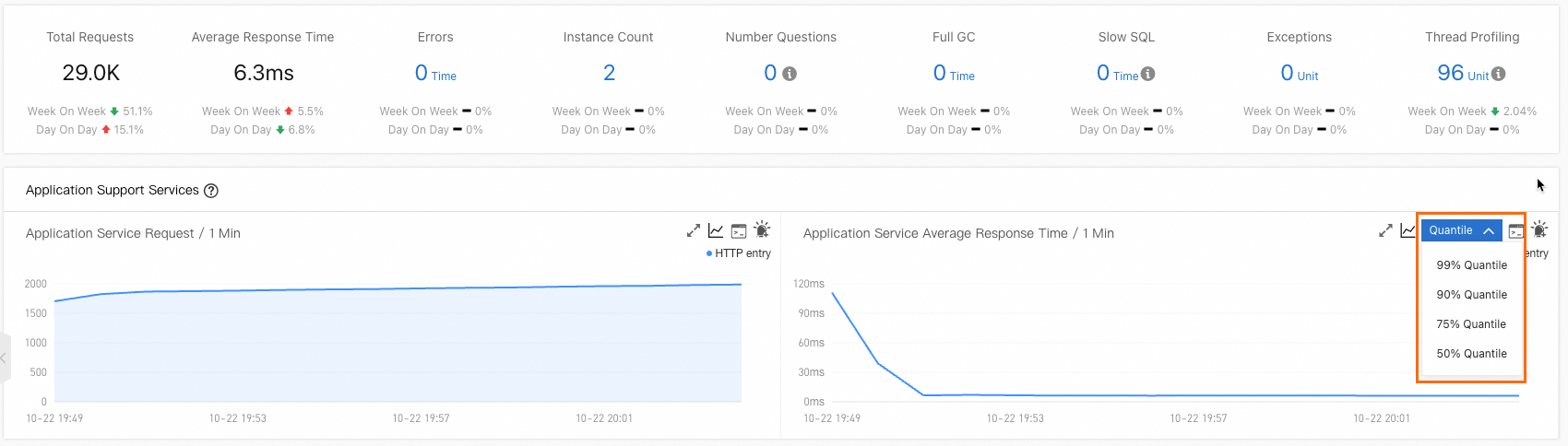
Enable quantile statistics
To collect quantile metrics, enable Quantile Statistics in the ARMS console.
New console
For details, see Customize settings for a Java application.
Old console
For details, see Customize application settings.
How the ARMS agent calculates quantiles
The ARMS agent (v4.x and later) calculates latency quantiles using a fixed-boundary histogram with linear interpolation. Instead of storing every individual latency value, the agent counts how many requests fall into each predefined bucket.
Bucket boundaries
The default bucket boundaries are (in milliseconds):
[0.0, 5.0, 10.0, 25.0, 50.0, 75.0, 100.0, 250.0, 500.0, 750.0, 1000.0, 2500.0, 5000.0, 7500.0, 10000.0]These boundaries create 16 buckets:
| Bucket | Range (ms) |
|---|---|
| 0 | (-Infinity, 0.0] |
| 1 | (0.0, 5.0] |
| 2 | (5.0, 10.0] |
| 3 | (10.0, 25.0] |
| 4 | (25.0, 50.0] |
| 5 | (50.0, 75.0] |
| 6 | (75.0, 100.0] |
| 7 | (100.0, 250.0] |
| 8 | (250.0, 500.0] |
| 9 | (500.0, 750.0] |
| 10 | (750.0, 1000.0] |
| 11 | (1000.0, 2500.0] |
| 12 | (2500.0, 5000.0] |
| 13 | (5000.0, 7500.0] |
| 14 | (7500.0, 10000.0] |
| 15 | (10000.0, +Infinity] |
Calculation steps
The calculation has two phases: bucket counting and linear interpolation.
Phase 1: Count requests per bucket
Each incoming request latency increments the counter of the bucket it falls into. Using the example data [2, 3, 6, 7, 8, 9, 10, 12, 14, 15, 16, 17, 18, 20]:
| Bucket | Range (ms) | Count | Values |
|---|---|---|---|
| 0 | (-Infinity, 0.0] | 0 | -- |
| 1 | (0.0, 5.0] | 2 | 2, 3 |
| 2 | (5.0, 10.0] | 5 | 6, 7, 8, 9, 10 |
| 3 | (10.0, 25.0] | 7 | 12, 14, 15, 16, 17, 18, 20 |
| 4-15 | (25.0, +Infinity] | 0 | -- |
Phase 2: Linear interpolation
To calculate a specific quantile, ARMS locates the target bucket and interpolates within it.
P75 walkthrough:
Find the target position. Total data points = 14. The P75 position is 14 x 0.75 = 10.5. ARMS rounds this up: the target cumulative count is 11.
Find the target bucket. Accumulate counts from left to right until the cumulative count reaches 11:
Bucket 0: cumulative = 0
Bucket 1: cumulative = 2
Bucket 2: cumulative = 7
Bucket 3: cumulative = 14 (first to reach 11) -- this is the target bucket.
Interpolate within the bucket. Buckets 0-2 already account for 7 data points. ARMS needs 4 more data points (11 - 7 = 4) from Bucket 3, which contains 7 data points total. Bucket 3 spans (10.0, 25.0]: P75 = 10.0 + (25.0 - 10.0) x 4 / 7 = 18.6
The exact P75 of the raw data is 16, but the histogram-based estimate is 18.6. This difference occurs because linear interpolation assumes data is uniformly distributed within a bucket, which is rarely the case. The wider the bucket, the larger the potential error.
Accuracy trade-offs
The fixed-boundary histogram approach is highly efficient but introduces estimation errors in certain scenarios.
Strengths
Low overhead. Only bucket counters are stored -- no need to keep every individual latency value in memory.
Limitations
In scenarios with extremely low latencies, extremely high latencies, or very few samples, the calculated quantiles may be inaccurate. Accuracy depends on how well the bucket boundaries match your actual latency distribution:
| Scenario | Impact | Why |
|---|---|---|
| Latencies concentrated in a wide bucket | Higher error | Linear interpolation assumes uniform distribution within the bucket, but actual data may be skewed. |
| Very low latencies (sub-millisecond) | Higher error | All sub-5 ms values land in a single 5 ms-wide bucket, reducing precision. |
| Very high latencies (above 10,000 ms) | Higher error | All values above 10,000 ms fall into the open-ended Bucket 15, making interpolation less reliable. |
| Very few samples | Higher error | With sparse data, the bucket a value lands in has an outsized impact on the result. |
| Latencies spread across narrow buckets | Lower error | The 5 ms and 10 ms-wide buckets at the low end provide finer granularity. |
How Trace Explorer calculates quantiles
Trace Explorer calculates quantiles based on the latencies of all spans that satisfy the page filtering conditions and the SQL functions of Simple Log Service. For more information, see the approx_percentile function in Function overview.