Optimize query performance with compound and interleaved sorting - AnalyticDB

AnalyticDB for PostgreSQL supports two sorting methods — compound sorting and interleaved sorting — to accelerate query performance. For most workloads, use compound sorting. Switch to interleaved sorting only when your queries filter on non-leading columns of the sort key with roughly equal frequency.

How sorting works

When you create a table, specify one or more columns as the sort key. After data is loaded, sort the table by the sort key. AnalyticDB for PostgreSQL records the minimum and maximum values for each column in every disk block, forming a rough set index. During a table scan, the query engine compares filter values against the min/max ranges and skips any disk blocks that fall outside the range.

Example: A table holds seven years of data sorted by date. A query for a single month needs to scan only 1/(7 × 12) of the data — 98.8% of disk blocks are skipped. Without sorting, the query scans every disk block.

Choose a sort key

For equality and range filters on a fixed set of columns, use compound sorting. Compound sorting treats the sort key as an ordered prefix: the query engine is most effective when filter conditions match the leading columns of the sort key. This is the right choice for the majority of queries.

For filters that span different, non-leading columns, use interleaved sorting. Interleaved sorting assigns equal weight to each column in the sort key, so the query engine can skip blocks regardless of which column appears in the filter. The trade-off is that interleaved sorting requires extra analysis on the data and is generally slower than compound sorting.

Note

An interleaved sort key can contain up to eight columns.

For JOIN columns, set the JOIN column as both the distribution key and the sort key. This lets the query optimizer choose a merge join instead of a hash join. Because the data is already sorted on the join key, the optimizer skips the sort phase of the merge join entirely.

Performance comparison between compound sorting and interleaved sorting

The following benchmark uses two columnar, append-only tables with identical data: test (sorted with SORT) and test_multi (sorted with MULTISORT). Both tables have the sort key (id, num1, num2).

Setup

Create both tables:

CREATE TABLE test(id int, num1 int, num2 int, value varchar)
WITH (APPENDONLY=TRUE, ORIENTATION=column)
DISTRIBUTED BY (id)
ORDER BY (id, num1, num2);

CREATE TABLE test_multi(id int, num1 int, num2 int, value varchar)
WITH (APPENDONLY=TRUE, ORIENTATION=column)
DISTRIBUTED BY (id)
ORDER BY (id, num1, num2);

Insert 10 million rows into each table:

INSERT INTO test(id, num1, num2, value)
SELECT g,
  (random() * 10000000)::int,
  (random() * 10000000)::int,
  (ARRAY['foo', 'bar', 'baz', 'quux', 'boy', 'girl', 'mouse', 'child', 'phone'])[floor(random() * 10 + 1)]
FROM generate_series(1, 10000000) AS g;

INSERT INTO test_multi SELECT * FROM test;

Sort each table using the corresponding method:

SORT test;            -- compound sorting
MULTISORT test_multi; -- interleaved sorting

Equality query results

Three queries filter on different combinations of sort key columns:

Q1 — first column only: WHERE id = 100000
Q2 — second column only: WHERE num1 = 8766963
Q3 — second and third columns: WHERE num1 = 100000 AND num2 = 2904114

Sorting method	Q1	Q2	Q3
Compound sorting	0.026 s	3.95 s	4.21 s
Interleaved sorting	0.55 s	0.42 s	0.071 s

Range query results

The same column combinations, using range predicates:

Q1 — first column: WHERE id > 5000 AND id < 100000
Q2 — second column: WHERE num1 > 5000 AND num1 < 100000
Q3 — second and third columns: WHERE num1 > 5000 AND num1 < 100000 AND num2 < 100000

Sorting method	Q1	Q2	Q3
Compound sorting	0.07 s	3.35 s	3.64 s
Interleaved sorting	0.44 s	0.28 s	0.047 s

Conclusions

Q1 (leading column filter): Compound sorting is faster. When the filter matches the leading column of the sort key, the query engine skips blocks efficiently without the extra analysis that interleaved sorting requires.
Q2 (non-leading column filter): Interleaved sorting outperforms compound sorting because it assigns independent min/max ranges to each column, not just the prefix.
Q3 (multiple non-leading columns): Interleaved sorting is significantly faster. The more non-leading columns included in the filter, the greater the advantage — each additional column contributes to narrowing the block scan.

Sorting acceleration

After you run SORT <tablename>, AnalyticDB for PostgreSQL pushes sort-aware operators — SORT, AGG, and JOIN — down to the storage layer. Queries that match the physical sort order of the data are executed against already-ordered blocks, eliminating in-flight sorting.

Note

Sorting acceleration requires all data in the table to be ordered. After writing new data, run SORT <tablename> again.
Sorting acceleration is enabled by default.

The following example compares query time before and after sorting acceleration on a test table named far.

Setup

Create the far table:

CREATE TABLE far(a int, b int)
WITH (APPENDONLY=TRUE, COMPRESSTYPE=ZSTD, COMPRESSLEVEL=5)
DISTRIBUTED BY (a)  -- distribution key
ORDER BY (a);       -- sort key

Insert one million rows:

INSERT INTO far VALUES (generate_series(0, 1000000), 1);

Sort the table:
```
SORT far;
```

Query performance comparison

Note

The query times below are for reference only. Actual times vary based on data volume, computing resources, and network conditions.

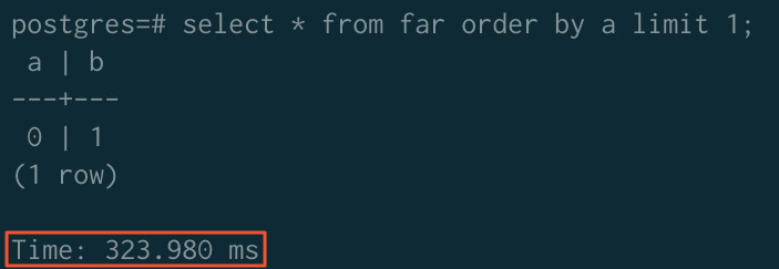
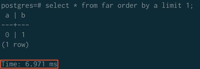
ORDER BY

Before sorting acceleration:
After sorting acceleration:

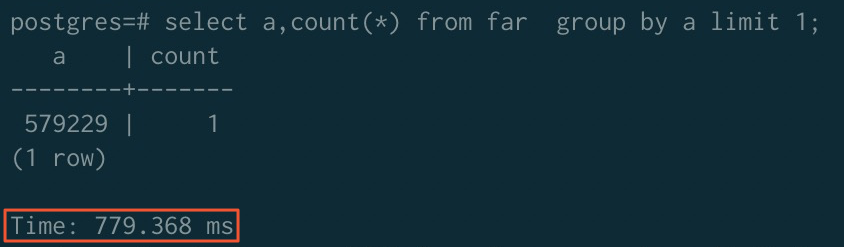
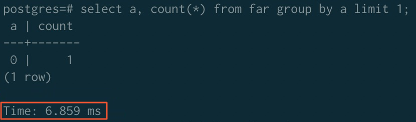
GROUP BY

Before sorting acceleration:
After sorting acceleration:

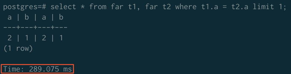
JOIN

Before sorting acceleration:
After sorting acceleration:
Note
To use sorting acceleration for JOIN operators, disable the ORCA optimizer and enable the merge join algorithm:
```
SET enable_mergejoin TO on;
SET optimizer TO off;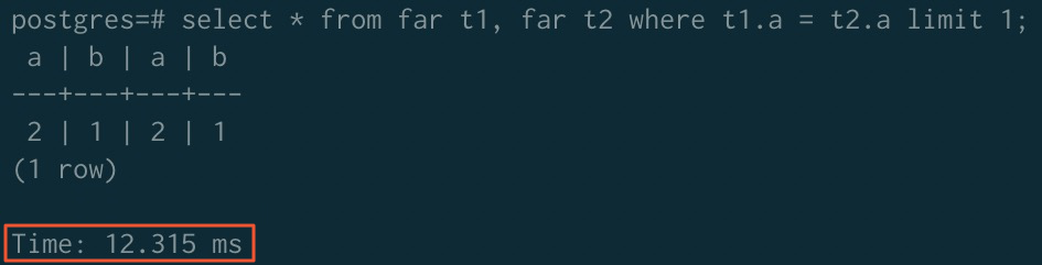
```

Summary

	ORDER BY	GROUP BY	JOIN
Before acceleration	323.980 ms	779.368 ms	289.075 ms
After acceleration	6.971 ms	6.859 ms	12.315 ms