AnalyticDB:Auto-scaling resource group evaluation

Multi-Cluster type

• Use cases: A Multi-Cluster resource group automatically scales resources up or down at the cluster level based on the group's load. It provides resource isolation within the group and is ideal for high-concurrency scenarios. It is suited for interactive queries where a single query's resource consumption does not exceed the capacity of one cluster. During peak business hours, it automatically provisions new compute nodes as clusters to increase overall computing capacity and adapt to the workload, preventing performance degradation. During off-peak hours, it automatically deprovisions compute nodes at the cluster level to reduce resource usage and save costs.

• Billing: For more information, see Billing Rules.

Job type

• Use cases: A Job resource group provisions temporary compute resources for a query and releases them immediately after the query finishes. It executes queries by using a Bulk Synchronous Parallel (BSP) model, resulting in response times of seconds to minutes. The amount of resources provisioned depends on the size of the running task. This type is ideal for non-real-time, resource-intensive tasks that are not latency-sensitive.

• Billing: For more information, see Billing Rules.

Auto-Scaling type

• Use cases: An Auto-Scaling resource group dynamically scales compute resources at the node level in real time based on the group's load. The maximum resources for a single query equal the resource group's upper limit. Provisioned compute nodes can be shared across multiple consecutive queries. This type provides resource isolation at the query level to prevent interference between queries and reduce performance fluctuations. It is ideal for mixed workloads that include both latency-sensitive interactive queries and resource-intensive batch queries.

• Billing: For more information, see Billing Rules.

Resource group comparison

Real-time queries—BI query performance

BI queries are one of the most common fixed workload types in a data warehouse. They typically involve predefined reports and dashboard queries executed by BI tools such as Tableau, PowerBI, or Quick BI. These queries have a clear business pattern: fixed SQL logic, high execution frequency (for scheduled refreshes or frequent access), and manageable result set sizes. They are mainly used for daily business monitoring, daily or weekly reports, and KPI dashboards. For BI queries, the core database requirements are stable concurrency and predictable latency. This ensures that dashboards do not lag when multiple users refresh them simultaneously during peak hours and that fixed reports are generated on time. Workload isolation is also important to prevent large queries from affecting the core reporting experience.

Using the 1 TB TPC-H dataset to simulate a BI query workload, we compared the performance of Auto-Scaling and Multi-Cluster resource groups under different concurrency levels. The results follow.

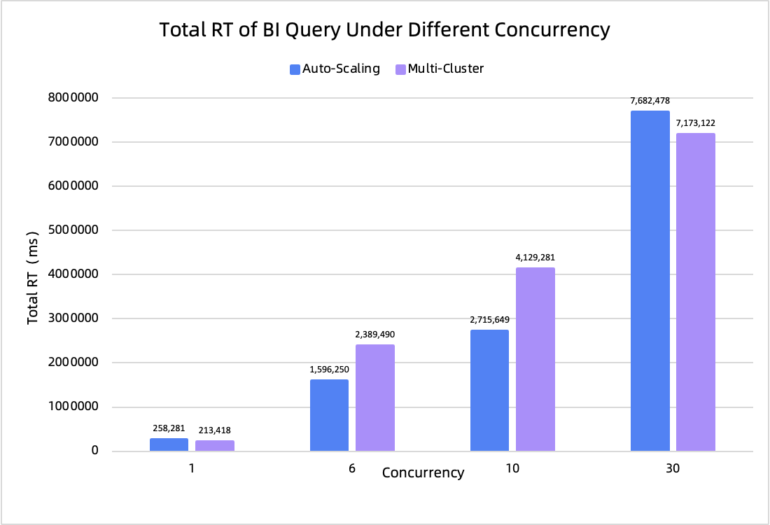
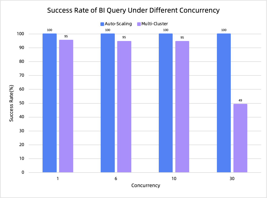
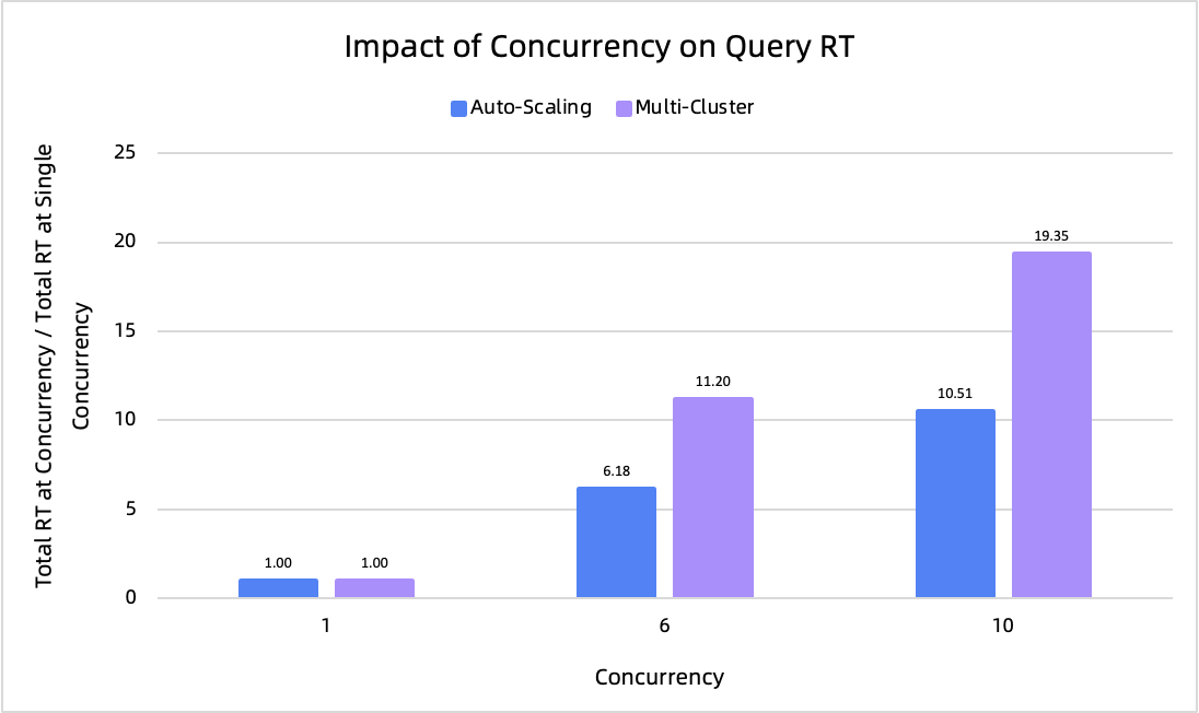
Test conclusion: The Auto-Scaling resource group achieved a 100% success rate for all queries across all concurrency levels. In contrast, the Multi-Cluster resource group experienced query failures, with a failure rate exceeding 50% at 30 concurrent queries. Excluding the 30-concurrency scenario where Multi-Cluster was nearly unusable, the test results for total response time (RT) show that as concurrency increases, the total RT for Auto-Scaling grows almost linearly, while Multi-Cluster's performance degrades significantly.

These results highlight the advantage of Auto-Scaling's query-level resource isolation. Even as concurrency increases, individual queries do not interfere with each other, ensuring both cluster availability and consistent query performance.

Real-time queries—Ad-hoc query performance

Ad-hoc queries are a typical exploratory workload in a data warehouse, often initiated by data analysts or business users for non-recurring analysis. These queries are highly unpredictable, with variable SQL logic (often handwritten or dynamically generated), high complexity (such as multi-table joins, nested subqueries, and complex aggregations), and widely fluctuating execution times. They are primarily used for data exploration, root cause analysis, and temporary data retrieval. For ad-hoc queries, a database must handle complex queries and high concurrency while providing fast response times to support interactive analysis.

Based on the TPC dataset, the following SQL statements were selected for testing:

• Lightweight ad-hoc: A set of queries with an approximate execution time of 5 seconds was created from the TPC dataset. These include multi-table joins for detailed retrieval, dimensional aggregation (GROUP BY + SUM/COUNT), ranking with window functions (RANK), multi-dimensional aggregation on a star schema, and top-N sorting of aggregated results. This set represents lightweight analytical tasks focused on quick browsing and summarization.

  Query SQL

  [
    {
      "sql": "SELECT c.c_name, o.o_orderdate, l.l_quantity FROM customer c JOIN orders o ON c.c_custkey = o.o_custkey JOIN lineitem l ON o.o_orderkey = l.l_orderkey LIMIT 100",
      "databaseName": "tpch_100g_iceberg",
      "description": "CONCURRENCY_ADHOC_1",
      "weight": 1.0,
      "queryType": "ADHOC"
    },
    {
      "sql": "SELECT p.p_brand, COUNT(*), SUM(l.l_extendedprice) FROM part p JOIN lineitem l ON p.p_partkey = l.l_partkey GROUP BY p.p_brand LIMIT 100",
      "databaseName": "tpch_100g_iceberg",
      "description": "CONCURRENCY_ADHOC_2",
      "weight": 1.0,
      "queryType": "ADHOC"
    },
    {
      "sql": "SELECT p_partkey, p_name, p_retailprice, RANK() OVER (ORDER BY p_retailprice DESC) as price_rank FROM part LIMIT 100",
      "databaseName": "tpch_100g_iceberg",
      "description": "CONCURRENCY_ADHOC_3",
      "weight": 1.0,
      "queryType": "ADHOC"
    },
    {
      "sql": "SELECT d.d_year, i.i_category, s.s_state, SUM(ss_sales_price) FROM store_sales ss JOIN date_dim d ON ss.ss_sold_date_sk = d.d_date_sk JOIN item i ON ss.ss_item_sk = i.i_item_sk JOIN store s ON ss.ss_store_sk = s.s_store_sk GROUP BY d.d_year, i.i_category, s.s_state LIMIT 100",
      "databaseName": "tpcds_100g_iceberg",
      "description": "CONCURRENCY_ADHOC_4",
      "weight": 1.0,
      "queryType": "ADHOC"
    },
    {
      "sql": "SELECT i.i_brand, COUNT(*), SUM(ss_sales_price), AVG(ss_sales_price) FROM store_sales ss JOIN item i ON ss.ss_item_sk = i.i_item_sk GROUP BY i.i_brand ORDER BY SUM(ss_sales_price) DESC LIMIT 50",
      "databaseName": "tpcds_100g_iceberg",
      "description": "CONCURRENCY_ADHOC_5",
      "weight": 1.0,
      "queryType": "ADHOC"
    }
  ]

• Complex ad-hoc: A set of queries with an approximate execution time of 10 seconds was created from the TPC dataset. These include semi-join filtering (EXISTS subquery), grouped comparisons with window functions (AVG OVER PARTITION BY), phased calculations with CTEs and top-N lookups, multi-dimensional aggregation on a star schema, and conditional segmentation with distinct counts (CASE + COUNT DISTINCT). This set represents heavyweight analytical tasks focused on in-depth exploration and segmentation.

  Query SQL

  [
    {
      "sql": "SELECT * FROM supplier s WHERE EXISTS (SELECT 1 FROM lineitem l WHERE l.l_suppkey = s.s_suppkey) LIMIT 100",
      "databaseName": "tpch_1t_iceberg",
      "description": "CONCURRENCY_ADHOC_1",
      "weight": 1.0,
      "queryType": "ADHOC"
    },
    {
      "sql": "SELECT o_custkey, o_totalprice, AVG(o_totalprice) OVER (PARTITION BY o_custkey) as customer_avg FROM orders LIMIT 100",
      "databaseName": "tpch_1t_iceberg",
      "description": "CONCURRENCY_ADHOC_2",
      "weight": 1.0,
      "queryType": "ADHOC"
    },
    {
      "sql": "WITH top_customers AS (SELECT c_custkey, SUM(o_totalprice) as total_spent FROM customer c JOIN orders o ON c.c_custkey = o.o_custkey GROUP BY c_custkey ORDER BY total_spent DESC LIMIT 10) SELECT tc.c_custkey, tc.total_spent, c.c_name, c.c_mktsegment FROM top_customers tc JOIN customer c ON tc.c_custkey = c.c_custkey LIMIT 100",
      "databaseName": "tpch_1t_iceberg",
      "description": "CONCURRENCY_ADHOC_3",
      "weight": 1.0,
      "queryType": "ADHOC"
    },
    {
      "sql": "SELECT d.d_year, i.i_category, s.s_state, SUM(ss_sales_price) FROM store_sales ss JOIN date_dim d ON ss.ss_sold_date_sk = d.d_date_sk JOIN item i ON ss.ss_item_sk = i.i_item_sk JOIN store s ON ss.ss_store_sk = s.s_store_sk GROUP BY d.d_year, i.i_category, s.s_state LIMIT 100",
      "databaseName": "tpcds_1t_iceberg",
      "description": "CONCURRENCY_ADHOC_4",
      "weight": 1.0,
      "queryType": "ADHOC"
    },
    {
      "sql": "SELECT CASE WHEN SUM(ss_sales_price) > 10000 THEN 'High Value' WHEN SUM(ss_sales_price) > 1000 THEN 'Medium Value' ELSE 'Low Value' END as customer_segment, COUNT(DISTINCT c.c_customer_sk) FROM store_sales ss JOIN customer c ON ss.ss_customer_sk = c.c_customer_sk GROUP BY c.c_customer_sk LIMIT 100",
      "databaseName": "tpcds_1t_iceberg",
      "description": "CONCURRENCY_ADHOC_5",
      "weight": 1.0,
      "queryType": "ADHOC"
    }
  ]

We tested the performance of Auto-Scaling and Multi-Cluster resource groups using these two sets of ad-hoc queries with 10, 20, 50, and 100 concurrent queries for five minutes each. The results follow.

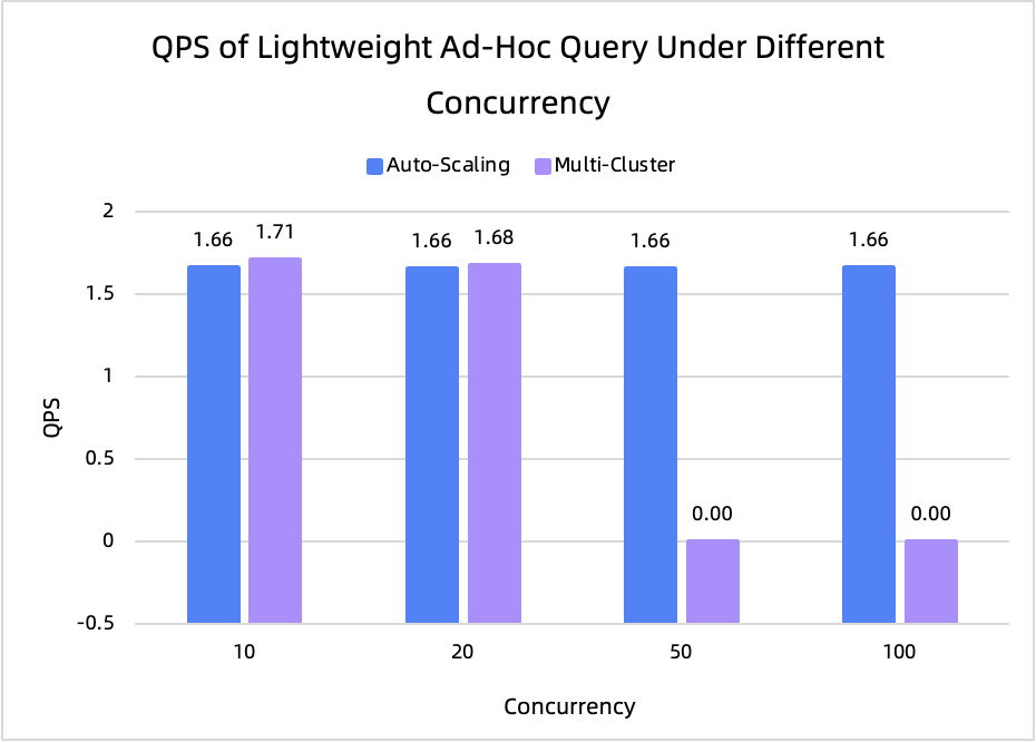
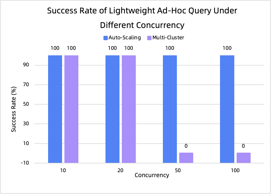
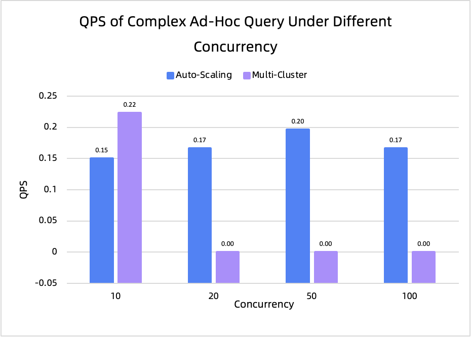
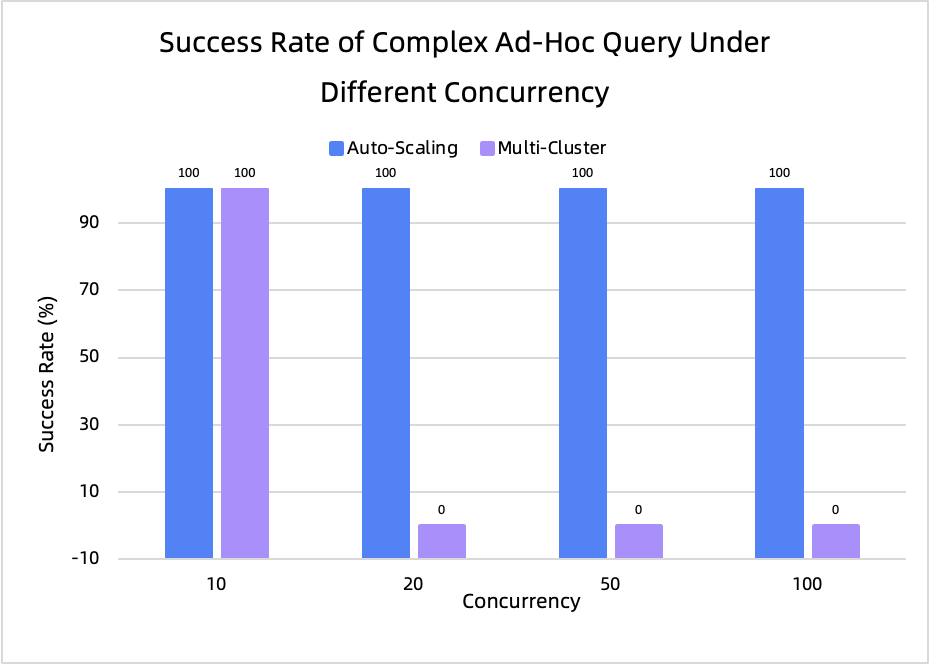
Test conclusion: The most significant finding from this test is that Auto-Scaling's availability under high concurrency is clearly superior to Multi-Cluster's. Starting at 50 concurrent queries, Multi-Cluster was unable to complete any lightweight ad-hoc queries within five minutes. For complex ad-hoc queries, Multi-Cluster became unresponsive at just 20 concurrent queries. Furthermore, observing the queries per second (QPS), Auto-Scaling maintained a stable QPS across different concurrency levels. This again demonstrates that Auto-Scaling provides excellent resource isolation between queries.

Real-time queries—Small query performance

Small queries are the most frequent type of query in many business scenarios. These queries consume few resources and are highly sensitive to latency and throughput. Based on the TPC dataset, we created two representative types of small queries: 1) distribution key point lookups, and 2) complex small queries.

A complex small query uses a highly selective filter to locate a small number of rows and then performs complex calculations, such as multi-table joins and multi-dimensional aggregation analysis. This query type simulates a typical online scenario of real-time user profile analysis.

-- Example 1: Real-time user profile analysis
SELECT
  SUM(
    CASE WHEN p.p_brand = 'Brand#12' THEN l.l_extendedprice ELSE 0 END
  ) AS brand12_sales,
  AVG(
    CASE WHEN p.p_brand = 'Brand#23' THEN l.l_extendedprice ELSE NULL END
  ) AS brand23_avg_price,
  SUM(
    CASE WHEN p.p_brand = 'Brand#34' THEN l.l_quantity ELSE 0 END
  ) AS brand34_quantity,
  AVG(
    CASE WHEN p.p_brand = 'Brand#45' THEN l.l_quantity ELSE NULL END
  ) AS brand45_avg_quantity,
  SUM(
    CASE WHEN p.p_brand = 'Brand#51' THEN l.l_extendedprice ELSE 0 END
  ) AS brand51_sales,
  AVG(
    CASE WHEN p.p_brand = 'Brand#13' THEN l.l_extendedprice ELSE NULL END
  ) AS brand13_avg_price,
  SUM(
    CASE WHEN p.p_brand = 'Brand#24' THEN l.l_quantity ELSE 0 END
  ) AS brand24_quantity,
  AVG(
    CASE WHEN p.p_brand = 'Brand#35' THEN l.l_quantity ELSE NULL END
  ) AS brand35_avg_quantity,
  SUM(
    CASE WHEN p.p_brand = 'Brand#41' THEN l.l_extendedprice ELSE 0 END
  ) AS brand41_sales,
  AVG(
    CASE WHEN p.p_brand = 'Brand#52' THEN l.l_extendedprice ELSE NULL END
  ) AS brand52_avg_price,
  SUM(
    CASE WHEN p.p_brand = 'Brand#14' THEN l.l_quantity ELSE 0 END
  ) AS brand14_quantity,
  AVG(
    CASE WHEN p.p_brand = 'Brand#25' THEN l.l_quantity ELSE NULL END
  ) AS brand25_avg_quantity,
  SUM(
    CASE WHEN p.p_brand = 'Brand#31' THEN l.l_extendedprice ELSE 0 END
  ) AS brand31_sales,
  AVG(
    CASE WHEN p.p_brand = 'Brand#42' THEN l.l_extendedprice ELSE NULL END
  ) AS brand42_avg_price,
  SUM(
    CASE WHEN p.p_brand = 'Brand#53' THEN l.l_quantity ELSE 0 END
  ) AS brand53_quantity
FROM
  orders o
  JOIN lineitem l ON o.o_orderkey = l.l_orderkey
  JOIN part p ON l.l_partkey = p.p_partkey
WHERE
  o.o_custkey = 135889;

-- Example 2: Multi-dimensional aggregation statistics
SELECT
    CAST(IFNULL(SUM(CASE WHEN i.i_current_price > 100 THEN 1 ELSE 0 END), 0) AS int) AS dx_expensive_items_cnt,
    CAST(IFNULL(MIN(CASE WHEN i.i_current_price > 100 THEN DATEDIFF(CURRENT_DATE, ss.ss_sold_date_sk) END), -99) AS int) AS dx_expensive_items_diff_days_min,
    CAST(IFNULL(COUNT(DISTINCT CASE WHEN i.i_current_price > 100 THEN i.i_category END), 0) AS int) AS dx_expensive_items_categories,
    CAST(IFNULL(SUM(CASE WHEN i.i_current_price > 100 AND DATEDIFF(CURRENT_DATE, ss.ss_sold_date_sk) < 14 THEN ss.ss_sales_price ELSE 0 END), 0) AS int) AS dx_expensive_items_14d_cnt,
    CAST(IFNULL(SUM(CASE WHEN i.i_current_price > 100 AND DATEDIFF(CURRENT_DATE, ss.ss_sold_date_sk) < 30 THEN ss.ss_sales_price ELSE 0 END), 0) AS int) AS dx_expensive_items_30d_cnt,
    CAST(IFNULL(SUM(CASE WHEN i.i_current_price > 100 AND DATEDIFF(CURRENT_DATE, ss.ss_sold_date_sk) < 60 THEN ss.ss_sales_price ELSE 0 END), 0) AS int) AS dx_expensive_items_60d_cnt,
    CAST(IFNULL(SUM(CASE WHEN i.i_current_price > 100 AND DATEDIFF(CURRENT_DATE, ss.ss_sold_date_sk) < 90 THEN ss.ss_sales_price ELSE 0 END), 0) AS int) AS dx_expensive_items_90d_cnt,
    c.c_customer_sk AS dx_expensive_group_rptid
FROM store_sales ss
JOIN item i ON ss.ss_item_sk = i.i_item_sk
JOIN customer c ON ss.ss_customer_sk = c.c_customer_sk
WHERE c.c_customer_sk = 10001
GROUP BY c.c_customer_sk
LIMIT 1;

The following charts show the performance of Auto-Scaling and Multi-Cluster resource groups for these two small query workloads under different concurrency levels.

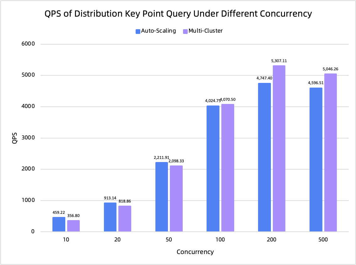
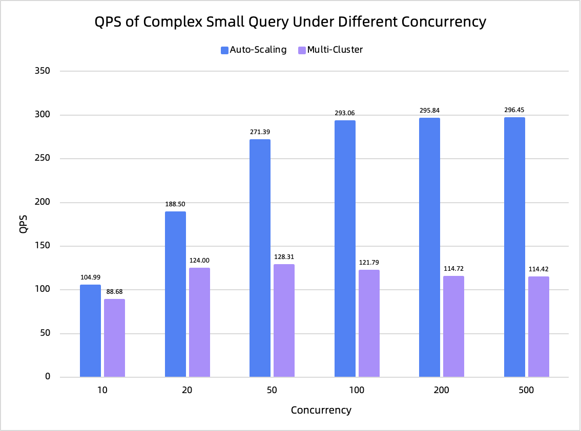
Test conclusion: In the distribution key point lookup scenario, Auto-Scaling's performance is slightly lower than Multi-Cluster's. However, in the complex small query scenario, Auto-Scaling demonstrates a clear advantage at high concurrency levels.

Offline query performance

Offline queries are a workload type in a data warehouse designed for batch data processing. They are typically used for non-real-time scenarios such as T+1 reporting, data warehouse layer processing, historical data archiving, and large-scale data analysis. These queries have distinct characteristics: terabyte- to petabyte-scale data volumes, execution times measured in hours, complex logic (multi-table joins, window functions, and aggregations), and low latency sensitivity but high stability requirements.

Using the 10 TB TPC dataset to simulate offline queries, we compared the performance of Auto-Scaling and Job resource groups.

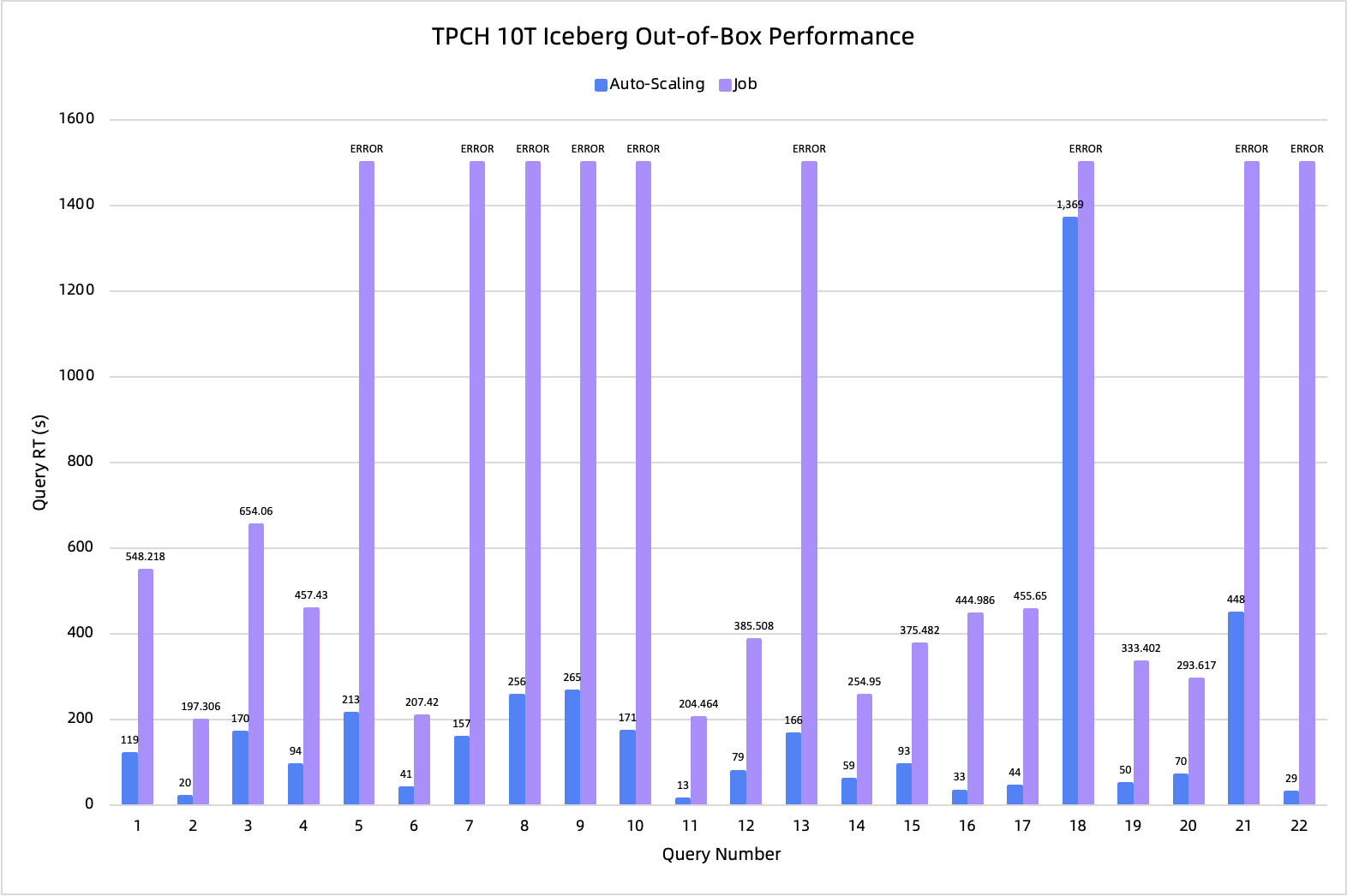
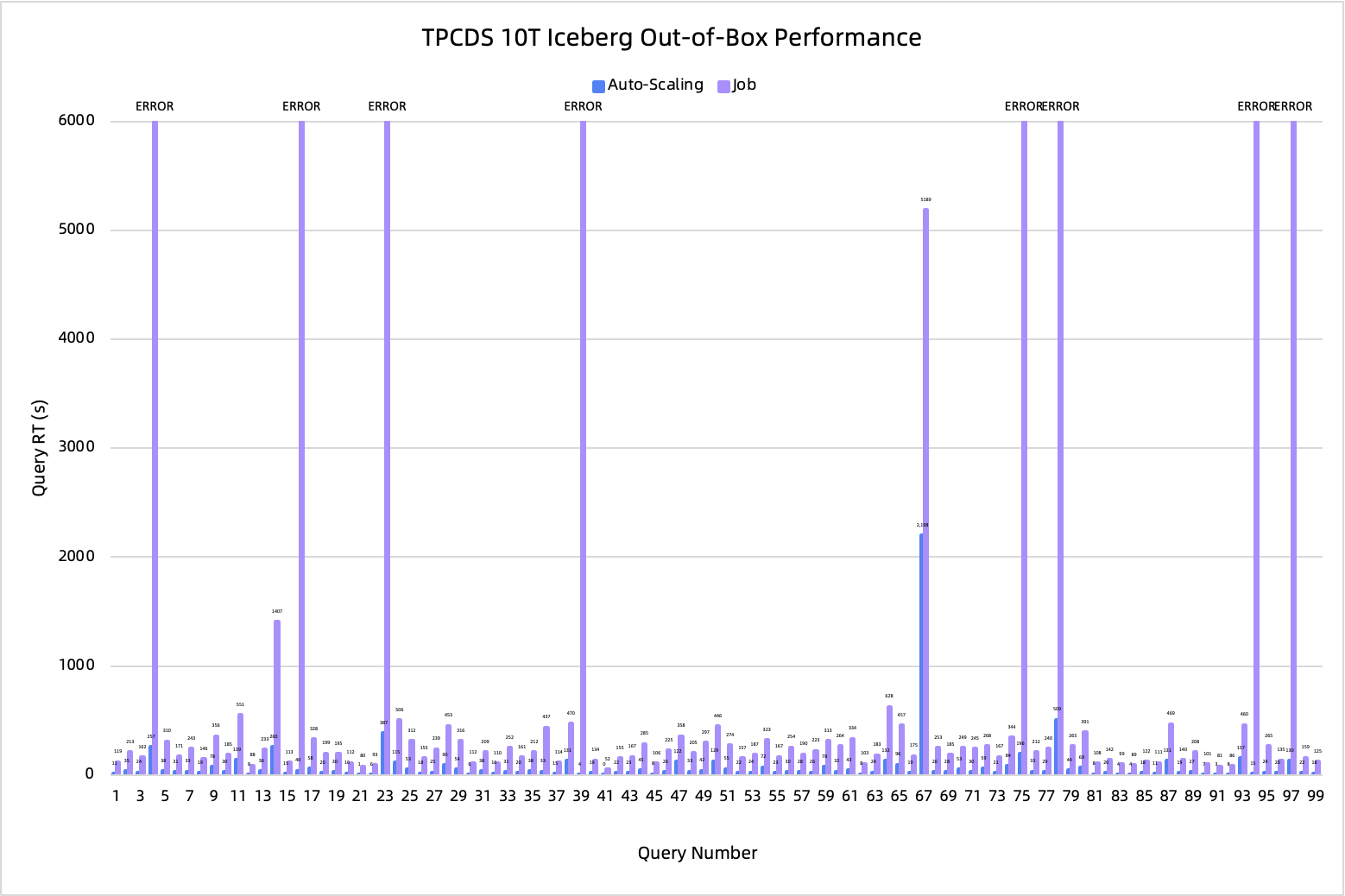
Test conclusion: In the TPC-H 10 TB out-of-the-box test, Auto-Scaling performed 443.44% better overall than the Job resource group. Auto-Scaling achieved a 100% success rate, while the Job resource group's success rate was only 59%. In the TPC-DS 10 TB out-of-the-box test, Auto-Scaling performed 355.17% better overall than the Job resource group. Again, Auto-Scaling achieved a 100% success rate, compared to 92% for the Job resource group. Therefore, in offline query scenarios, Auto-Scaling is significantly superior to the Job resource group in both query performance and stability.

Capability matrix

The following table summarizes the performance of the three resource group types across various evaluation dimensions:

Evaluation summary

Key conclusions

• Auto-Scaling matches and exceeds Multi-Cluster in real-time query scenarios: In high-concurrency scenarios such as BI queries, ad-hoc queries, and complex small queries, Auto-Scaling delivers superior stability and a higher query success rate at high concurrency, thanks to its query-level resource isolation. While the failure rate of Multi-Cluster increases significantly under high concurrency, Auto-Scaling consistently maintains a 100% success rate.

• Auto-Scaling outperforms Job in offline query scenarios: In offline query scenarios, Auto-Scaling is overwhelmingly superior to the Job resource group in both query performance and stability.

• Key advantages of Auto-Scaling:

  • Query-level resource isolation: Allocates and isolates resources at the query level, preventing interference between queries and ensuring stable performance under high concurrency.

  • Fully pay-as-you-go: Unlike Multi-Cluster, which bills for a minimum of one cluster, Auto-Scaling bills only for the resources consumed.

  • Node-level elastic scaling: Scales resources at the node level, providing more fine-grained elasticity than the cluster-level scaling of Multi-Cluster.

  • One resource group for multiple scenarios: Supports both interactive and batch queries, eliminating the need for multiple resource groups.

• Recommendation: Auto-Scaling is recommended for mixed workloads (both real-time and offline queries), high-concurrency real-time query scenarios, and cost-sensitive scenarios.