From Common Crawl to Training-Ready Corpora: Cleaning, Annotation & Vectorization with EMR Serverless Daft

EMR Serverless Daft enables end-to-end web corpus processing in a single DataFrame pipeline — from WARC extraction through cleaning, deduplication, LL...

Introduction

Before raw web pages can feed LLM pretraining, fine-tuning, or a RAG index, they typically go through main-content extraction, normalization, quality filtering, deduplication, model-based annotation, and vectorization. The algorithms themselves are not mysterious — the hard part is keeping these very different kinds of computation running stably on large-scale data, and being able to adjust thresholds, swap models, or add new fields without rewriting the whole pipeline.

Alibaba Cloud EMR Serverless Spark ships a build of Daft that is integrated with and optimized for the serverless environment. Daft is a distributed DataFrame engine for multimodal data; EMR Serverless Daft goes further with operators for text cleaning, media processing, and document parsing, and brings LLM generation and embedding service calls into the DataFrame execution plan through ai_query and ai_embedding. As a result, "read WARC → extract content → score quality → deduplicate → annotate with an LLM → generate vectors → write to OSS" can be expressed in a single DataFrame pipeline. The table below first shows where these capabilities sit along the corpus pipeline.

The Product Capabilities This Pipeline Covers

Pipeline stage	EMR Serverless Daft capability	Example used in this article	Main output
Data ingestion and content extraction	OSS data access, WARC/HTML parsing	`CommonCrawlContentExtractor`, `HtmlTagRemover`	URL, main text, source file
Cleaning and quality signals	Batch text operators, model reuse	Whitespace normalization, regex replacement, repetition and perplexity	Cleaned text, quality features
Deduplication	Hash expressions, MinHash, shuffle and graph-compute pipelines	Exact dedup + MinHash/LSH near-duplicate dedup	Unique documents or representative samples
LLM calls	Concurrency, batching, rate-limit backoff, token accounting	`ai_query`	Categories, labels, JSON extraction results
Vectorization	Batched embedding service calls	`ai_embedding`	Vectors, token usage, model name
Delivery	DataFrame write to OSS Parquet	`write_parquet`	Training datasets or vector-store import files

The rest of this article walks one concrete pipeline from end to end: the input is a set of Common Crawl WARC files on OSS, and the output is an English corpus ready for training or vector retrieval. The sample thresholds are only a starting point — in production, recalibrate them by language, source, and downstream task using sampling and offline evaluation.

What the Major Public Corpus Pipelines Do

Public large-scale web corpus efforts differ in the details, but they broadly share the same stages: heuristic filtering, deduplication, and language- or model-based quality assessment.

C4 applies heuristic cleaning rules to Common Crawl; the MassiveWeb data processing in the Gopher paper contributes filtering signals such as document length, bullet lines, repeated lines, and repeated n-grams; RefinedWeb demonstrates the value of large-scale web filtering and deduplication; CCNet combines document deduplication, language identification, and quality bucketing driven by Wikipedia language models; FineWeb and FineWeb-Edu systematically evaluate filtering and deduplication strategies and use an educational-quality classifier to select a subset.

Stacking these practices together gives a six-stage pipeline:

Content extraction: pull human-readable main text out of WARC / HTML, dropping navigation bars, ads, scripts, and styles.
Normalization: unify whitespace, redact sensitive data, and strip copyright headers and boilerplate text.
Heuristic filtering: use a set of cheap statistics to remove obviously low-quality pages.
Deduplication: exact dedup removes fully identical documents, while MinHash near-duplicate dedup identifies near-identical documents with heavily overlapping n-grams.
Model-based quality scoring: use a statistical language model or a classifier to assess linguistic well-formedness, information density, or domain fit.
Vectorization and ingestion: the retrieval path produces vectors and loads them into a vector database such as Milvus; the training path writes the text out as Parquet directly.

These public efforts are a reference for methods, not a set of thresholds that can be reused unconditionally. The same rule produces different distributions on English news, Chinese forums, and code documentation. What actually consumes engineering effort is running stably at scale, retaining intermediate signals, and iterating on strategy quickly.

Why EMR Serverless Daft for This Pipeline

Scale. The full Common Crawl dataset is petabyte-scale, and WARC files contain a large number of HTTP response records. Content extraction is CPU-intensive, and the runtime of a single-machine script grows quickly with data volume.

Ecosystem fragmentation. Content extraction needs Python libraries such as trafilatura / jusText / goose3; quality scoring needs to load a fastText model; perplexity needs KenLM and SentencePiece; annotation and vectorization need calls to LLM services, with concurrency, rate limiting, and retries all hand-rolled. Each dependency carries its own loading cost, and a naive UDF wrapper re-initializes the model in every task.

Fault tolerance. Web data quality is wildly uneven: truncated HTML, wrong encodings, and binary content disguised as HTML all show up. One bad record can rerun an entire partition and wipe out hours of computation.

Composition and governance. Every statistic needs stable input/output types, null semantics, model paths, and error boundaries. If every pipeline wraps its own UDFs, algorithm versions, thresholds, and error handling quickly fork.

Scheduling. The cleaning stage is CPU-intensive and wants high parallelism, while LLM calls such as annotation and vectorization go over the network and need bounded concurrency and rate-limit handling. Put both in the same DAG and how do you allocate resources?

The built-in operator library of EMR Serverless Daft exists to solve exactly this layer of engineering problems. The sections below follow the pipeline and show how to write it.

Stage 1: From WARC to One Row per Document

Assume there is a batch of .warc.gz files on OSS — either synced from Common Crawl or written by an in-house crawler. CommonCrawlContentExtractor expands them into structured records:

import daft
from daft import col
from daft.emr.functions import CommonCrawlContentExtractor, emr_udf

EXTRACT_CONCURRENCY = 64  # Sample value; tune to the number of WARC files and available cluster CPUs.

docs = (
    daft.from_glob_path("oss://my-bucket/crawl/CC-MAIN-2025-33/*.warc.gz")
    # Explicitly split input partitions so WARC files can be processed by multiple extractors in parallel.
    .into_partitions(EXTRACT_CONCURRENCY)
    .with_column(
        "records",
        emr_udf(
            CommonCrawlContentExtractor,
            construct_args={
                "warc_src_type": "warc_url",     # warc_binary / warc_url / warc_base64
                "extractor_type": "trafilatura", # trafilatura / justext / goose3
            },
            num_cpus=2,
            concurrency=EXTRACT_CONCURRENCY,
            batch_size=1,
        )(warc_files=col("path")),
    )
    .explode("records")
    .select(
        col("records").get("url").alias("url"),
        col("records").get("content").alias("raw_text"),
        col("records").get("warc_file").alias("warc_file"),
    )
    .where(col("raw_text").not_null())
)

Internally, the operator iterates WARC records with warcio, keeps only entries whose WARC-Type is response, decodes the HTTP response body as UTF-8 (decode errors fall back to replacement characters), and hands the result to the selected extraction backend. One input row (one WARC file) produces a list[struct]; the struct carries four fields — url, content, warc_file, and extractor — and after explode you get one row per document. warc_file records the source file name (the basename of the path when warc_src_type="warc_url", an empty string in the other input modes), so keep a separate column with the original path if you need the full path.

The trade-offs among the three extraction backends deserve a note. trafilatura is the operator's default and was also used by RefinedWeb for web content extraction; justext detects boilerplate at the paragraph level using stopword density; goose3 targets main-content extraction from article-style pages. No backend is optimal for every site — sample by domain and page type, compare content recall, template residue, and empty-result rates, and then choose.

If the input is already a column of HTML — site snapshots, internal document libraries, pages fetched from APIs — skip the WARC layer and use HtmlTagRemover directly:

from daft.emr.functions import HtmlTagRemover, emr_udf

df = df.with_column(
    "raw_text",
    emr_udf(
        HtmlTagRemover,
        construct_args={"separator": "\n", "strip": True},
        num_cpus=1,
        concurrency=32,
        batch_size=512,
    )(texts=col("html")),
)

HtmlTagRemover is designed around "plain text meant for a large model to read", not simply deleting angle brackets: <script> / <style> / <head> / <title> / <noscript> / <template> are removed together with their inner text, and comments and DOCTYPE are ignored; block-level elements such as <div> / <p> / <h1> through <h6> / <li> / <table>are split into separate text segments joined by separator — pass "\n" and each block gets its own line; inline tags such as <b> / <strong> / <a> cause no split, so <p>First <b>bold</b> end</p> still comes out as one complete sentence; indentation and newlines inside <pre> are preserved as-is with only the outermost whitespace trimmed, so the original formatting of code blocks survives. Parsing runs in lenient mode: unclosed tags and fragments missing an <html> / <body> wrapper still extract correctly.

Stage 2: Clean the Noise While Preserving Line Structure

After content extraction, first apply regex replacement and copyright-notice cleaning and store the result as text_lines. This column keeps newlines and exists specifically to compute the repeated-line and bullet-line ratios. Then apply WhitespaceNormalizer to turn Unicode whitespace (including newlines) into ASCII spaces, producing the single-line text used for hashing, n-grams, model scoring, and embeddings.

[!warning] Do not flatten line breaks before computing line-level signals WhitespaceNormalizer turns \n into a space too. If you normalize first and then call RepeatedLinesCalculator or BulletLineRatioCalculator, the document usually collapses to a single line and the results become meaningless.

from daft.emr.functions import (
    CopyrightCleaner,
    RegexReplacer,
    WhitespaceNormalizer,
    emr_udf,
)

cleaned = (
    docs
    .with_column(
        "text_lines",
        emr_udf(
            RegexReplacer,
            construct_args={
                "patterns": [
                    r"[\w.+-]+@[\w-]+\.[\w.]+",              # Email addresses
                    r"(?<!\d)\+?\d[\d\-\s]{7,}\d(?!\d)",     # Phone numbers
                ],
                "replacements": ["<EMAIL>", "<PHONE>"],
            },
            num_cpus=1,
            concurrency=32,
            batch_size=512,
        )(texts=col("raw_text")),
    )
    .with_column(
        "text_lines",
        emr_udf(CopyrightCleaner, num_cpus=1, concurrency=32, batch_size=512)(
            texts=col("text_lines")
        ),
    )
    .with_column(
        "text",
        emr_udf(WhitespaceNormalizer, num_cpus=1, concurrency=32, batch_size=512)(
            texts=col("text_lines")
        ),
    )
)

RegexReplacer supports a broadcast style in which "multiple patterns share one replacement string": when replacements has a single element, it is automatically expanded across all patterns. A malformed regex is skipped with a warning instead of failing the whole job.

[!important] Cleaning is not the same as compliance The email and phone regexes above are pipeline examples and cannot cover all personal data. CopyrightCleaner only removes specific marked comments, and that does not mean the content is licensed. A production corpus still requires independent data-source review, privacy redaction, content safety, takedown handling, and license governance.

Stage 3: Compute All Quality Signals in One Pass

This stage corresponds to the heuristic rules of Gopher and C4. EMR Serverless Daft packages each statistic as an independent operator that can be composed as needed:

Operator	Actual output	Purpose	Sample threshold
`TextLengthCalculator`	Int64, number of Unicode characters	Filter overly short or long text; not equivalent to filtering by "word count"	200 to 500,000
`RepeatedLinesCalculator`	Float64, extra occurrences of repeated lines / non-empty lines	Detect template lines, repeated menus, and repeated paragraphs	< 0.30
`WordRepetitionCalculator`	Float64, share of n-gram instances that keep recurring	Detect phrase stuffing and template repetition	5-gram < 0.15
`BulletLineRatioCalculator`	Float64, share of bullet lines	Detect menu, navigation, or list-style pages	< 0.90
`UrlRatioCalculator`	Float64, URL character coverage	Detect link-dense pages	< 0.20
`AlphanumericRatioCalculator`	Float64, share of characters that are Unicode letters or digits	Detect symbol- or garbage-dense text; not "share of words containing letters"	> 0.70
`MaximumWordLengthCalculator`	Int64, longest English word length	Detect base64, hash strings, or garbage fragments	≤ 40

from daft.emr.functions import (
    AlphanumericRatioCalculator,
    BulletLineRatioCalculator,
    MaximumWordLengthCalculator,
    RepeatedLinesCalculator,
    TextLengthCalculator,
    UrlRatioCalculator,
    WordRepetitionCalculator,
    emr_udf,
)

POOL = dict(num_cpus=1, concurrency=32, batch_size=1024)

signals = (
    cleaned
    .with_column("n_chars", emr_udf(TextLengthCalculator, **POOL)(texts=col("text")))
    .with_column("dup_line_ratio", emr_udf(RepeatedLinesCalculator, **POOL)(texts=col("text_lines")))
    .with_column(
        "dup_5gram_ratio",
        emr_udf(
            WordRepetitionCalculator,
            construct_args={"repetition": 5, "lang": "en", "tokenization": False},
            **POOL,
        )(texts=col("text")),
    )
    .with_column("bullet_ratio", emr_udf(BulletLineRatioCalculator, **POOL)(texts=col("text_lines")))
    .with_column("url_ratio", emr_udf(UrlRatioCalculator, **POOL)(texts=col("text")))
    .with_column("alnum_ratio", emr_udf(AlphanumericRatioCalculator, **POOL)(texts=col("text")))
    .with_column("max_word_len", emr_udf(MaximumWordLengthCalculator, **POOL)(texts=col("text")))
)

candidate = signals.where(
    (col("n_chars") >= 200)
    & (col("n_chars") <= 500_000)
    & (col("dup_line_ratio") < 0.30)
    & (col("dup_5gram_ratio") < 0.15)
    & (col("bullet_ratio") < 0.90)
    & (col("url_ratio") < 0.20)
    & (col("alnum_ratio") > 0.70)
    & (col("max_word_len") <= 40)
)

A more robust production pattern is: compute and persist all quality signals first, then apply the filter conditions as a separate step. Look at the feature distributions across source, language, and time partition first, then calibrate thresholds with manual sampling and downstream evaluation. The candidate above only demonstrates the filter expression; if you need explainability, persist signals first.

One parameter of WordRepetitionCalculator deserves attention: with tokenization=True it loads a SentencePiece model for tokenization, which is required for Chinese; for a pure English corpus, tokenization=False splits on whitespace directly, dropping the model dependency and running faster.

Stage 4: Deduplicate First, Then Spend on Unique Content

Deduplication sits before remote LLM calls and vectorization for a straightforward reason: the same content should not consume tokens and embedding requests twice. The actual reduction depends on crawl scope, time span, normalization rules, and the near-duplicate threshold, so do not promise a fixed reduction without baseline data. Deduplication happens in two steps: exact deduplication first, then MinHash + LSH to catch lexical near-duplicates.

Exact dedup: hash the normalized text, then take distinct on the fingerprint. The hash must be computed on the normalized text, not the raw extracted text — after whitespace normalization, email/phone masking, and copyright cleanup, copies that differ only in formatting land on the same fingerprint. Hash first, then deduplicate by fingerprint, is also the approach taken by CCNet and FineWeb. Daft's hash expression computes a 64-bit integer fingerprint per text (xxhash3 by default), which combined with a row-level distinct completes the job in two steps:

exact = candidate.with_column("text_hash", col("text").hash()).distinct("text_hash")

hash() is for fast grouping, not cryptographic hashing. For data with audit or strict-correctness requirements, compare the normalized texts within the same hash group and explicitly choose a representative row by time, source priority, or text completeness rather than relying on the arbitrary survivor of distinct.

Exact dedup removes copies that are identical after normalization. The remaining near-duplicates may differ by only a few templates, ads, or sentences, and can be identified with MinHash signatures and LSH candidate sets. MinHash estimates n-gram set similarity — it is not semantic deduplication and may not catch heavy rewrites or cross-language paraphrases. Daft ships MinHash as a built-in expression:

sig = exact.with_column(
    "min_hashes",
    col("text").minhash(
        num_hashes=128,
        ngram_size=5,
        seed=1,
        hash_function="xxhash",
    ),
)

After the signatures, you still need LSH bucketing, candidate-pair construction, connected components, and representative-sample selection. For that part, see the official Daft MinHash deduplication tutorial. To keep the variable names below unambiguous, this article uses deduped for the DataFrame after near-duplicate deduplication; if you only need exact deduplication for now, continue with the baseline below:

# Baseline: skip LSH near-duplicate dedup for now
# In a production pipeline, replace this line with the representative-sample DataFrame produced by the official tutorial.
deduped = exact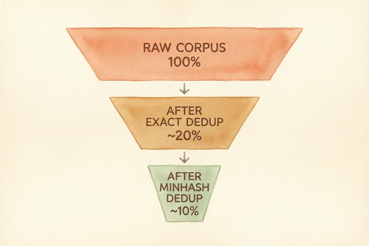

The two-step ordering is a cost decision: exact dedup is a hash plus a shuffle, usually cheaper than MinHash signatures, LSH bucketing, and connected components. Running it first shrinks the candidate set and cuts the compute and shuffle cost of the near-duplicate stage. Record per-stage input row count, output row count, retention rate, and the largest duplicate cluster in a run report, and evaluate the value of deduplication against real data.

Stage 5: Model-Based Quality Scoring

Rules filter out obviously low-quality content, but not text that is "grammatically correct yet carries little information". That job goes to two lightweight models. By this point the data is already deduplicated and only representative samples need scoring, which avoids paying inference costs repeatedly for duplicate content.

EnTextQualityScorer uses the fastText classifier kenhktsui/llm-data-textbook-quality-fasttext-classifier-v2 and outputs a continuous score between 0 and 2. It computes the probability-weighted expectation over the Low(0) / Mid(1) / High(2) classes, so it can drive ranking, quantile splitting, or threshold filtering. A higher score means the classifier leans toward judging the text as textbook or popular-science content; 0.5 works as an initial observation point, but it is not a universal quality standard. This model runs on CPU.

PerplexityCalculator follows the CCNet recipe: SentencePiece tokenization first, then a KenLM n-gram model trained on Wikipedia scores the text line by line, and the per-line log probabilities and word counts are accumulated into a single perplexity value for the whole document. Lower perplexity means the text is closer to the standard written prose found on Wikipedia. Both Chinese and English are supported.

from daft.emr.functions import EnTextQualityScorer, PerplexityCalculator, emr_udf

scored = (
    deduped
    .with_column(
        "quality_score",
        emr_udf(
            EnTextQualityScorer,
            construct_args={
                "model_path": "oss://my-bucket/models",  # Downloaded automatically to local cache on first use
                "batch_size": 64,
            },
            num_cpus=1,
            concurrency=32,
            batch_size=512,
        )(texts=col("text")),
    )
    .with_column(
        "ppl",
        emr_udf(
            PerplexityCalculator,
            construct_args={"lang": "en", "model_path": "/opt/emr/models"},
            num_cpus=1,
            concurrency=32,
            batch_size=512,
        )(texts=col("text")),
    )
)

high_quality = scored.where(
    col("quality_score").not_null()
    & col("ppl").not_null()
    & (col("quality_score") > 0.5)
    & (col("ppl") < 1000)
)

The two scores capture different signals: perplexity measures how close the text is to the current KenLM reference distribution, while the quality score reflects the educational-content preference learned by the fastText classifier. Keep both for analysis, but do not treat both thresholds as hard filters before evaluating the false-positive rate. Documents dense in formulas, code, and specialized terminology can produce high perplexity while still being valuable for specific training tasks.

One easily missed deployment detail: the model_path of EnTextQualityScorer accepts the oss:// prefix — the specified model files are downloaded to a local cache on initialization and reused afterwards. The KenLM and SentencePiece assets used by PerplexityCalculator load from a local model directory whose default base path is /opt/emr/models.

A reminder: EnTextQualityScorer is an English classifier, so in multilingual scenarios run language identification first and route only English text into this operator. EMR Serverless Daft also provides LanguageRecognizer, based on the fastText lid.176 model, which outputs a language code and a confidence score and can be used to split the flow early in the pipeline.

Stage 6: Semantic Enrichment and Vectorization

At this point the corpus is clean; what remains is shaping it into a form that downstream jobs can consume directly.

ai_query: Batch LLM Classification, Labeling, and Extraction in a DataFrame

ai_query takes a per-row text prompt, with optional image or video columns. In a corpus pipeline, typical uses include domain classification, boilerplate detection, safety labels, summarization, and structured information extraction. Models can be routed through the AI-function default configuration in EMR Serverless, a service_name, or an explicit model; the models actually available depend on the current workspace and model-service configuration.

For domain labeling, use ai_query and treat the LLM call as an ordinary DataFrame expression:

from daft import lit
from daft.emr.functions import ai_query

tagged = high_quality.with_column(
    "ai_result",
    ai_query(
        lit(
            "Read the passage and reply with JSON only, fields: "
            "domain (science / code / news / forum / commerce / other), "
            "is_boilerplate (true or false).\n\n"
        )
        + col("text"),
        model="qwen3.6-plus",
        concurrency=8,
        batch_size=64,
        options={"temperature": 0, "max_tokens": 128},
    ),
).with_column("domain_json", col("ai_result").get("content"))

ai_query returns a struct whose fields include content, reasoning_content, finish_reason, prompt_tokens, completion_tokens, total_tokens, cached_tokens, reasoning_tokens, model, id, and error. These fields make it easy to account for tokens and model-response metadata. The domain_json in the example above is still a string — downstream should validate it against a JSON schema instead of trusting the prompt to guarantee well-formed output.

A service call that still fails after retries fails the job; do not assume every failure is silently converted into a row-level error. Production pipelines should pair this with idempotent output paths, partition reruns, and run monitoring.

[!tip] Chunk first, then call the model Web page text can exceed the model's context window or the per-request input limit of the embedding service. Before ai_query and ai_embedding, chunk by heading, paragraph, or token count, and keep document_id, chunk_id, and the source URL.

ai_embedding: Turn a Text Column into Vectors in Batch

ai_embedding calls the configured embedding service through an OpenAI-compatible embeddings interface and packs multiple rows into batch requests. It returns a struct containing embedding, prompt_tokens, completion_tokens, total_tokens, model, and error. Empty strings and nulls are not sent to the service and come back as empty vectors; non-empty requests that still fail after retries raise an error.

from daft.emr.functions import ai_embedding

final = (
    tagged
    .with_column(
        "emb",
        ai_embedding(
            col("text"),
            concurrency=8,
            batch_size=256,
            embedding_batch_size=8,
        ),
    )
    .with_column("vector", col("emb").get("embedding"))
)
final.write_parquet("oss://my-bucket/corpus/en-clean/")

What gets persisted depends on how it will be consumed. Pretraining data usually keeps the text, source, language, quality score, and filter version, without pre-generating vectors; RAG and semantic-retrieval scenarios should keep the chunk text, vectors, primary keys, and traceable metadata. Parquet works well as the intermediate delivery format on OSS, with index files generated later to match the import spec of the target vector database.

What the Built-In Operators Buy You

When writing the pipeline, you make the business-level decisions: which extraction backend to use, which quality signals to compute, how to calibrate thresholds, which model to call, and which traceable fields to keep. The operators uniformly carry the engineering semantics — batch interfaces, resource declarations, model loading, and service concurrency.

The point of this encapsulation is collapsing complex logic into simple operator calls. The content-extraction operator handles WARC iteration, encoding fallback, and degraded error recording internally; the quality-scoring operators handle model loading, cache distribution, and batch inference; what you see in pipeline code is one expression and a few business parameters. The person writing the code faces the business — what to extract, what to keep, how to score — not the implementation details of every stage.

Error boundaries differ by operator type: a single failed extraction inside a WARC can degrade to empty content, several text-scoring operators return nulls for invalid rows, and model-service requests fail the job once retries are exhausted. This separation avoids swallowing all errors indiscriminately and keeps data-quality issues distinguishable from systemic ones.

The remote-model operators also expose separate knobs for row batch size, requests packed per call, in-job concurrency, and the service request window. You can therefore tune throughput against model-service rate limits and per-text size without touching the business expression.

Closing Thoughts

Every stage of corpus cleaning has a mature reference method. The genuinely hard part is making extraction, quality assessment, deduplication, model calls, and vectorization share one observable, traceable, iterable data flow.

The core value of Alibaba Cloud EMR Serverless Daft is combining batch unstructured-data processing with model-service calls such as ai_query and ai_embedding in a single DataFrame job. For teams that already keep raw data on OSS and want to build LLM training corpora or RAG indexes in batch, it offers a composable engineering path.

Contact Us

Want to see how EMR powers elastic, fully managed big data analytics with Spark, StarRocks, Ray, and lakehouse-native AI? 👉 Try EMR on Alibaba Cloud or talk to our solution architect to explore how you can build data lakes, real-time warehouses, and Data + AI workflows with seamless scalability.

More Resources：

E-MapReduce Document

E-MapReduce Serverless Spark Free Trial:1000 CU*H 3 months !

Community

From Common Crawl to Training-Ready Corpora: Cleaning, Annotation & Vectorization with EMR Serverless Daft

Introduction

The Product Capabilities This Pipeline Covers

What the Major Public Corpus Pipelines Do

Why EMR Serverless Daft for This Pipeline

Stage 1: From WARC to One Row per Document

Stage 2: Clean the Noise While Preserving Line Structure

Stage 3: Compute All Quality Signals in One Pass

Stage 4: Deduplicate First, Then Spend on Unique Content

Stage 5: Model-Based Quality Scoring

Stage 6: Semantic Enrichment and Vectorization

ai_query: Batch LLM Classification, Labeling, and Extraction in a DataFrame

ai_embedding: Turn a Text Column into Vectors in Batch

What the Built-In Operators Buy You

Closing Thoughts

Contact Us

Read previous post:

Alibaba Cloud Big Data and AI

You may also like

Comments

Alibaba Cloud Big Data and AI

Related Products

Big Data Consulting for Data Technology Solution

Big Data Consulting Services for Retail Solution

Quick BI

ApsaraDB for HBase