本文介紹了計劃加速(PartitionedTable Scan)的功能背景、使用方法以及效能對比等內容。
背景
PolarDB PostgreSQL版(相容Oracle)對分區表的分區數量沒有限制。當分區超過2級時,分區數量便會成倍增加。
例如,一個分區表有兩級分區,一級分區按照雜湊分割,有100個分區;二級分區按照雜湊分割,每個二級分區再次分成100個子分區。此時整個分區表共有10000個分區。此時如果對這個分區表進行查詢,查詢計劃如下:
explain analyze select * from part_hash;
                                 QUERY PLAN
-----------------------------------------------------------------------------
 Append  (cost=0.00..344500.00 rows=16300000 width=22)
   ->  Seq Scan on part_hash_sys0102  (cost=0.00..26.30 rows=1630 width=22)
   ->  Seq Scan on part_hash_sys0103  (cost=0.00..26.30 rows=1630 width=22)
   ->  Seq Scan on part_hash_sys0104  (cost=0.00..26.30 rows=1630 width=22)
  ...
  ...
  ...
   ->  Seq Scan on part_hash_sys10198  (cost=0.00..26.30 rows=1630 width=22)
   ->  Seq Scan on part_hash_sys10199  (cost=0.00..26.30 rows=1630 width=22)
   ->  Seq Scan on part_hash_sys10200  (cost=0.00..26.30 rows=1630 width=22)
 Planning Time: 3183.644 ms
 Execution Time: 633.779 ms
(10003 rows)
Total Memory: 216852KB從上述結果可以看到,查詢過程比較緩慢。這是因為分區表在最佳化器中的原理可以簡單理解為:首先對每個分區產生最優的Plan,然後使用Append運算元把這些Plan並聯起來作為分區表的最優Plan。如果分區表的分區數量較少,這個過程會很快,對於使用者是無感知的;但是一旦達到一定規模的分區數,這個過程變得逐漸明顯,使用者在查詢過程中感到分區表的查詢相比於普通表尤為緩慢。
如上面的SQL中,表part_hash有10000個分區,它的Planning Time可以達到3秒左右,但普通表的查詢Planning Time僅需0.1毫秒,達到了幾百倍的差距。並且除了Planning Time上的差距,查詢進程記憶體的佔用也非常巨大,可能會引發OOM。
分區表的這個缺陷在使用串連查詢時更加明顯:
create table part_hash2 (a int, b int, c varchar(10))
PARTITION by HASH(a) SUBPARTITION by HASH (b) PARTITIONS 100 SUBPARTITIONS 100;

explain analyze select count(*) from part_hash a join part_hash2 b on a.a=b.b where b.c = '0001';
                                                                            QUERY PLAN
-------------------------------------------------------------------------------------------------------------------------------------------------------------------
 Finalize Aggregate  (cost=48970442.90..48970442.91 rows=1 width=8) (actual time=6466.854..6859.935 rows=1 loops=1)
   ->  Gather  (cost=48970442.68..48970442.89 rows=2 width=8) (actual time=397.780..6859.902 rows=3 loops=1)
         Workers Planned: 2
         Workers Launched: 2
         ->  Partial Aggregate  (cost=48969442.68..48969442.69 rows=1 width=8) (actual time=4.748..11.768 rows=1 loops=3)
               ->  Merge Join  (cost=1403826.01..42177776.01 rows=2716666667 width=0) (actual time=4.736..11.756 rows=0 loops=3)
                     Merge Cond: (a.a = b.b)
                     ->  Sort  (cost=1093160.93..1110135.93 rows=6790000 width=4) (actual time=4.734..8.588 rows=0 loops=3)
                           Sort Key: a.a
                           Sort Method: quicksort  Memory: 25kB
                           Worker 0:  Sort Method: quicksort  Memory: 25kB
                           Worker 1:  Sort Method: quicksort  Memory: 25kB
                           ->  Parallel Append  (cost=0.00..229832.35 rows=6790000 width=4) (actual time=4.665..8.518 rows=0 loops=3)
                                 ->  Parallel Seq Scan on part_hash_sys0102 a  (cost=0.00..19.59 rows=959 width=4) (actual time=0.001..0.001 rows=0 loops=1)
                                 ->  Parallel Seq Scan on part_hash_sys0103 a_1  (cost=0.00..19.59 rows=959 width=4) (actual time=0.001..0.001 rows=0 loops=1)
                                 ->  Parallel Seq Scan on part_hash_sys0104 a_2  (cost=0.00..19.59 rows=959 width=4) (actual time=0.001..0.001 rows=0 loops=1)
                                  ...
                     ->  Sort  (cost=310665.08..310865.08 rows=80000 width=4) (never executed)
                           Sort Key: b.b
                           ->  Append  (cost=0.00..304150.00 rows=80000 width=4) (never executed)
                                 ->  Seq Scan on part_hash2_sys0102 b  (cost=0.00..30.38 rows=8 width=4) (never executed)
                                       Filter: ((c)::text = '0001'::text)
                                 ->  Seq Scan on part_hash2_sys0103 b_1  (cost=0.00..30.38 rows=8 width=4) (never executed)
                                       Filter: ((c)::text = '0001'::text)
                                 ->  Seq Scan on part_hash2_sys0104 b_2  (cost=0.00..30.38 rows=8 width=4) (never executed)
                                       Filter: ((c)::text = '0001'::text)
                                  ...

 Planning Time: 221082.616 ms
 Execution Time: 9500.148 ms
(30018 rows)
Total Memory: 679540KB
因此我們可以看到分區表在進行全表查詢時,因為沒有指定任何限定條件,無法將查詢集中在某個分區內,這導致在全表查詢情境下,分區表所有的優勢不再存在,比普通表更加低效。儘管我們可以通過分區剪枝使查詢可以集中在少部分分區,但是對於一些OLAP情境,必須對整個分區表進行全表掃描。
概述
為瞭解決這個問題,提供了PartitionedTableScan運算元。它是一個分區表的查詢運算元,比Append更加高效,可以明顯降低Planning Time,且使用更少的記憶體,有效避免OOM。該運算元用於解決分區表分區數量過多時,查詢效能慢的問題。
下方展示了當使用PartitionedTableScan運算元時,分別查詢這兩個SQL所用的Planning Time和記憶體。
explain analyze select * from part_hash;
                                 QUERY PLAN
----------------------------------------------------------------------------------------------------------------------------------------------------
PartitionedTableScan on part_hash  (cost=0.00..1.00 rows=1 width=22) (actual time=134.348..134.352 rows=0 loops=1)(Iteration partition number 10000)
   Scan Partitions: part_hash_sys0102, part_hash_sys0103, ...part_hash_sys10198, part_hash_sys10199, part_hash_sys10200
   ->  Seq Scan on part_hash  (cost=0.00..1.00 rows=1 width=22)
 Planning Time: 293.778 ms
 Execution Time: 384.202 ms
(5 rows)
Total Memory: 40276KB

explain analyze select count(*) from part_hash a join part_hash2 b on a.a=b.b where b.c = '0001';
                                                                            QUERY PLAN
-------------------------------------------------------------------------------------------------------------------------------------------------------------------
Aggregate  (cost=2.02..2.03 rows=1 width=8) (actual time=152.322..152.326 rows=1 loops=1)
   ->  Nested Loop  (cost=0.00..2.02 rows=1 width=0) (actual time=152.308..152.311 rows=0 loops=1)
         Join Filter: (a.a = b.b)
         ->  PartitionedTableScan on part_hash a  (cost=0.00..1.00 rows=1 width=4) (actual time=152.305..152.306 rows=0 loops=1)(Iteration partition number 10000)
               Scan Partitions: part_hash_sys0102, part_hash_sys0103,, part_hash_sys10198, part_hash_sys10199, part_hash_sys10200
               ->  Seq Scan on part_hash a  (cost=0.00..1.00 rows=1 width=4)
         ->  PartitionedTableScan on part_hash2 b  (cost=0.00..1.00 rows=1 width=4) (never executed)
               ->  Seq Scan on part_hash2 b  (cost=0.00..1.00 rows=1 width=4)
                     Filter: ((c)::text = '0001'::text)
 Planning Time: 732.952 ms
 Execution Time: 436.927 ms
(11 rows)
Total Memory: 68104KB可以看到,在本樣本中,不管是Planning Time 還是記憶體Total Memory,使用PartitionedTableScan運算元後都顯著下降。具體數字對比樣本如下表:
類型 |
|
|
Single Query Planning Time | 3183.644ms | 293.778ms |
Single Total Memory | 216852 KB | 40276 KB |
Join Query Planning Time | 221082.616ms | 732.952ms |
Join Total Memory | 679540 KB | 68104 KB |
使用限制
PolarDB PostgreSQL版(相容Oracle)1.0和2.0都支援
PartitionedTableScan運算元。且核心小版本需為V1.1.32及以上。PartitionedTableScan目前僅支援Select,不支援DML語句。PartitionedTableScan不支援分區串連。如果您開啟了分區串連功能,將不會產生PartitionedTableScan計劃。
PartitionedTable Scan功能僅適用於核心小版本為V1.1.32及以上的叢集。若早於該核心小版本的存量叢集需要使用該功能,請聯絡我們進行開啟。
使用說明
為了更好的說明PartitionedTableScan功能,我們結合如下樣本來進行介紹。
首先建立一張分區表。
CREATE TABLE prt1 (a int, b int, c varchar) PARTITION BY Hash(a) partitions 16;通過參數啟用PartitionedTableScan
通過對參數polar_num_parts_for_partitionedscan的設定調整,可以開啟或關閉PartitionedTableScan功能。
參數 | 取值範圍 | 預設值 | 說明 |
polar_num_parts_for_partitionedscan | -1至INT_MAX | 64 | 表示 例如,當為預設值時,即表示當分區表的子分區數量大於64時,自動開啟 該參數有如下兩個特殊取值:
|
樣本如下:
SET polar_num_parts_for_partitionedscan to -1;
explain select * from prt1;
                           QUERY PLAN
-----------------------------------------------------------------
 PartitionedTableScan on prt1  (cost=0.00..1.00 rows=1 width=40)
   ->  Seq Scan on prt1  (cost=0.00..1.00 rows=1 width=40)
(2 rows)
使用HINT
使用HINT文法PARTEDSCAN(table alias),樣本如下:
EXPLAIN select /*+PARTEDSCAN(prt1) */ select * from prt1;
                           QUERY PLAN
-----------------------------------------------------------------
 PartitionedTableScan on prt1  (cost=0.00..1.00 rows=1 width=40)
   ->  Seq Scan on prt1  (cost=0.00..1.00 rows=1 width=40)
(2 rows)
並行查詢
支援分區表的並行查詢,它能很好的處理大規模資料的查詢。和Append一樣,PartitionedTableScan也支援並行查詢。但和Append不同的是,PartitionedTableScan的並行查詢被稱之為PartitionedTableScan Append,並行的方式只有兩種:分區間並行和混合并行。
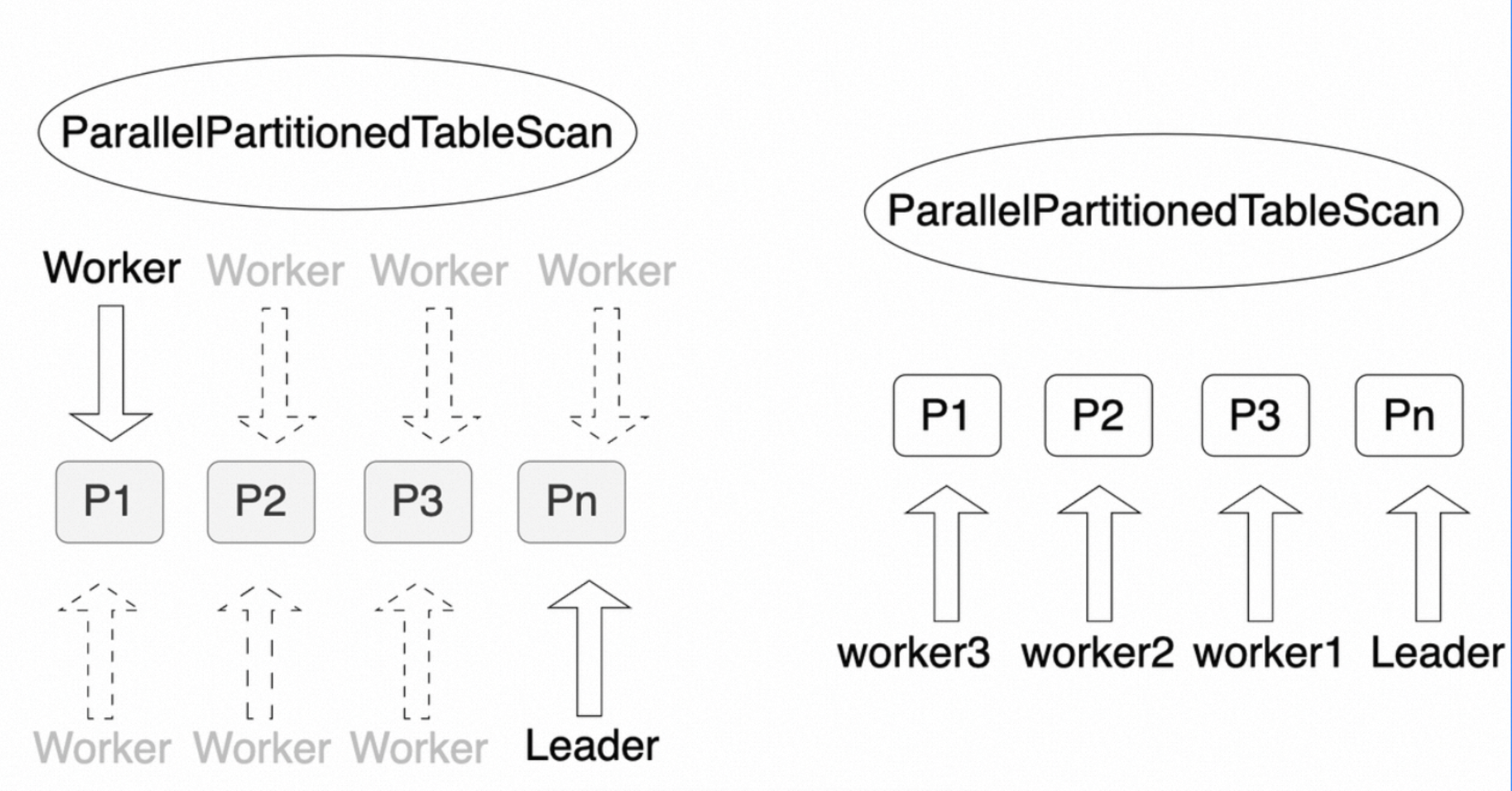
分區間並行
分區間並行是指每個worker查詢一個分區,以實現多個worker並行查詢整個分區表。
EXPLAIN (COSTS OFF) select /*+PARTEDSCAN(prt1) */ * from prt1;
                 QUERY PLAN
---------------------------------------------
 Gather
   Workers Planned: 4
   ->  Parallel PartitionedTableScan on prt1
         ->  Seq Scan on prt1
(4 rows)
如上所示,整個分區表啟動了4個並行的Worker(Workers Planned: 4),每個Worker負責查詢一個分區。其中,明顯的標誌是有一個名為Parallel PartitionedTableScan的運算元。
混合并行
混合并行是指分區間和分區內都可以並存執行,從而達到分區表整體的並存執行,這是並行度最高的一種並行查詢。
EXPLAIN (COSTS OFF) select /*+PARTEDSCAN(prt1) */ * from prt1;
                 QUERY PLAN
---------------------------------------------
 Gather
   Workers Planned: 8
   ->  Parallel PartitionedTableScan on prt1
         ->  Parallel Seq Scan on prt1
(4 rows)
如上所示,整個查詢使用了8個worker進行並行查詢(Workers Planned: 8),每個分區之間可以並行查詢,每個分區內部也可以並行查詢。其中,明顯的標誌是有一個名為Parallel PartitionedTableScan的運算元。
以上兩種並行方式都有自己的代價模型,最佳化器會選擇最優的一種。
分區剪枝
PartitionedTableScan和Append一樣,支援三個階段的分區剪枝。關於分區剪枝的詳細說明,請參見分區剪枝。
效能對比
PartitionedTableScan相比於Append更加高效。如下測試資料展示了PartitionedTableScan和Append的效能對比。
以下測試資料是開發環境測試出的臨時資料,不是效能標準資料。不同配置、不同條件下測試出的資料可能不同。本測試的目的是根據單一變數原則,在環境配置一致的情況下,對比Append和PartitionedTableScan的效能差異。
如下為測試SQL:
explain select  * from prt1 where b = 10;

explain select /*+PARTEDSCAN(prt1) */ * from prt1 where b = 10;
單條SQL的Planning Time
分區數量 | Append Planning Time | PartitionedTableScan Planning Time |
16 | 0.266ms | 0.067ms |
32 | 1.820ms | 0.258ms |
64 | 3.654ms | 0.402ms |
128 | 7.010ms | 0.664ms |
256 | 14.095ms | 1.247ms |
512 | 27.697ms | 2.328ms |
1024 | 73.176ms | 4.165ms |
Memory(單條SQL的記憶體使用量量)
分區數量 | Append Memory | PartitionedTableScan Memory |
16 | 1,170 KB | 1,044 KB |
32 | 1,240 KB | 1,044 KB |
64 | 2,120 KB | 1,624 KB |
128 | 2,244 KB | 1,524 KB |
256 | 2,888 KB | 2,072 KB |
512 | 4,720 KB | 3,012 KB |
1024 | 8,236 KB | 5,280 KB |
QPS(Query per Second)
pgbench -i --scale=10
pgbench -c 64 -j 64 -n -T60
Query:
	explain select  * from prt1 where b = 10;
	explain select /*+PARTEDSCAN(prt1) */ * from prt1 where b = 10;
分區數量 | Append QPS | PartitionedTableScan QPS |
16 | 25,318 | 93,950 |
32 | 10,906 | 61,879 |
64 | 5,281 | 30,839 |
128 | 2,195 | 16,684 |
256 | 920 | 8,372 |
512 | 92 | 3,708 |
1024 | 21 | 1,190 |
結論
從上面的PartitionedTableScan和Append的對比可以看出,PartitionedTableScan相比於Append隨著分區數量增加時,效能提升明顯。因此,如果您在業務中分區表分區數量較多且Planning Time很大時,我們建議您使用PartitionedTableScan進行一定程度的最佳化。