Simple Log Service:SQL syntax and functions

Simple Log Service allows you to analyze data in the search results by using SQL statements. This topic describes the basic syntax of SQL analytic statements.

Basic syntax

Search statement|Analytic statement

* | SELECT status, count(*) AS PV GROUP BY status

SQL functions and SQL clauses

In most cases, SQL functions are used to calculate, convert, and format data. For more information, see SQL functions. For example, you can use SQL functions to calculate the sum and average of values, perform operations on strings, and process dates. In most cases, SQL functions are embedded in SQL clauses.

SQL clauses are used to create complete SQL search statements or data processing statements to identify the sources, conditions, groups, and orders of data. For more information, see SQL clauses.

Example 1. Query logs of the previous day

The current_date function returns the current date. The date_add function subtracts a specific interval from the current date. The results are displayed in a table, which allows you to view data in an intuitive manner. (Demo)

• Query statement

  * |
  SELECT
    *
  FROM  log
  WHERE
    __time__ < to_unixtime(current_date)
    AND __time__ > to_unixtime(date_add('day', -1, current_date))

• Results

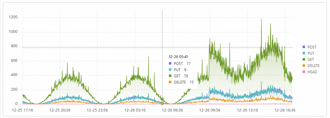
Example 2. Query the distribution of source IP addresses for logs

The ip_to_province function returns the provinces by IP address. The GROUP BY clause aggregates the provinces. Then, the count function calculates the number of requests from each province. The results are displayed in a pie chart. (Demo)

• Query statement

  * |
  select  
    count(1) as c,
    ip_to_province(remote_addr) as address
  group by
    address
  limit
    100

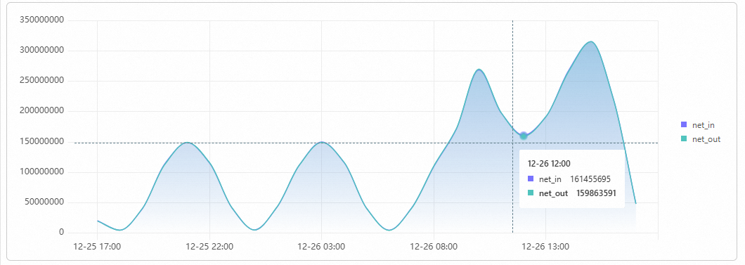
Example 3. Query the inbound and outbound NGINX traffic

The date_trunc function truncates the values of the __time__ field by hour. The __time__ field is a system field that specifies the log collection time. The default value of the __time__ field is a timestamp that is accurate to the second. The date_format function formats the truncated time values. The GROUP BY clause aggregates the time values. The sum function calculates the total volume of traffic per hour. The results are displayed in a line chart, in which the x-axis is set to time and the y-axis on the left is set to net_out and net_in. (Demo)

• Query statement

  * |
  select
    sum(body_bytes_sent) as net_out,
    sum(request_length) as net_in,
    date_format(date_trunc('hour', __time__), '%m-%d %H:%i') as time
  group by
    date_format(date_trunc('hour', __time__), '%m-%d %H:%i')
  order by
    time
  limit
    10000

• Results

  

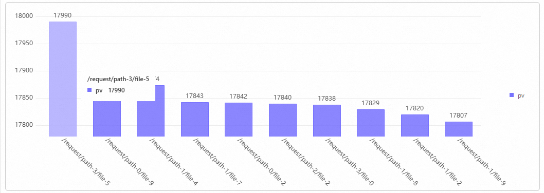
Example 4. Query the top 10 most accessed URLs in NGINX

The split_part function splits the request_uri field into arrays by using the question mark (?) and obtains the request paths from the first string of the arrays. The GROUP BY clause aggregates the request paths. The count function calculates the number of times that each path is accessed. The ORDER BY clause sorts the paths in descending order based on the number of times that each path is accessed. The results are displayed in a column chart. (Demo)

• Query statement

  * |
  select
    count(1) as pv,
    split_part(request_uri, '?', 1) as path
  group by
    path
  order by
    pv desc
  limit
    10

• Results

  

Example 5. Query the category and PV trend of request methods

The date_trunc function truncates time values by minute. The GROUP BY clause aggregates and groups the truncated time values to calculate the number of page views (PVs) by request_method. The ORDER BY clause sorts the time values in ascending order. The results are displayed in a flow chart. In the chart, the x-axis indicates time values and the y-axis indicates the number of PVs. The aggregate column is request_method. (Demo)

• Query statement

  * |
  select
    date_format(date_trunc('minute', __time__), '%m-%d %H:%i') as t,
    request_method,
    count(*) as pv
  group by
    t,
    request_method
  order by
    t asc
  limit
    10000

• Results

  

Example 6. Query the number of PVs for the current day and the day-over-day comparison in PVs between the current day and the previous day

The count function calculates the number of PVs for the current day. The compare function returns the day-over-day comparison in PVs between the current day and the previous day. (Demo)

• Query statement

  * |
  select
    diff [1] as today,
    round((diff [3] -1.0) * 100, 2) as growth
  FROM
    (
      SELECT
        compare(pv, 86400) as diff
      FROM
        (
          SELECT
            COUNT(1) as pv
          FROM
            log
        )
    )

• Results

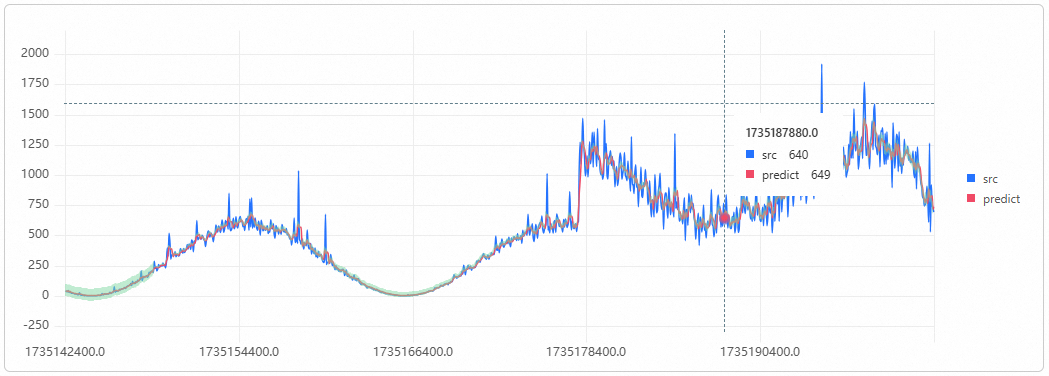
Example 7. Forecast the number of PVs based on NGINX access logs

The time - time % 60 expression subtracts the remainder of time values divided by 60 from the time values to obtain timestamps that are accurate to the minute. The GROUP BY clause aggregates the timestamps. The count function calculates the number of PVs per minute and the results are used as the subquery in a new query. The ts_predicate_simple function forecasts the number of PVs within the next 6 minutes. The results are displayed in a time series chart. (Demo)

• Query statement

  * |
  select
    ts_predicate_simple(stamp, value, 6)
  from
    (
      select
        __time__ - __time__ % 60 as stamp,
        COUNT(1) as value
      from
        log
      GROUP BY
        stamp
      order by
        stamp
    )
  LIMIT
    1000

• Results

  

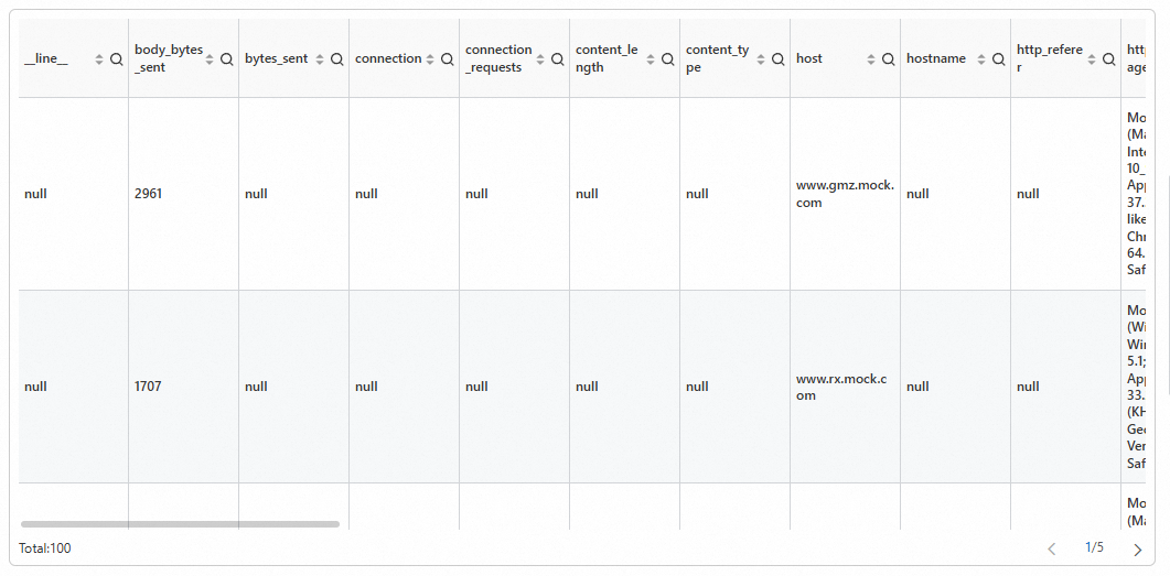
Example 8. Collect data based on the http_user_agent field, and sort and display the data by the number of PVs

The data is grouped and aggregated based on the http_user_agent field. The number of requests from each agent and the total response size returned to the clients are queried. The unit of the total response size is bytes. The round function converts the size in bytes to the size in MB and rounds the size to two decimal places. The CASE WHEN expression categorizes the status string into layers, including 2xx, 3xx, 4xx, and 5xx, and calculates the percentage of each layer. The results are displayed in a table, which allows you to view the data and the meanings of the data in an intuitive manner. (Demo)

• Query statement

  * |
  select
    http_user_agent as "User agent",
    count(*) as pv,
    round(sum(request_length) / 1024.0 / 1024, 2) as "Request traffic (MB)",
    round(sum(body_bytes_sent) / 1024.0 / 1024, 2) as "Response traffic (MB)",
    round(
      sum(
        case
          when status >= 200
          and status < 300 then 1
          else 0
        end
      ) * 100.0 / count(1),
      6
    ) as "Percentage of status code 2xx (%)",
    round(
      sum(
        case
          when status >= 300
          and status < 400 then 1
          else 0
        end
      ) * 100.0 / count(1),
      6
    ) as "Percentage of status code 3xx (%)",
    round(
      sum(
        case
          when status >= 400
          and status < 500 then 1
          else 0
        end
      ) * 100.0 / count(1),
      6
    ) as "Percentage of status code 4xx (%)",
    round(
      sum(
        case
          when status >= 500
          and status < 600 then 1
          else 0
        end
      ) * 100.0 / count(1),
      6
    ) as "Percentage of status code 5xx (%)"
  group by
    "User agent"
  order by
    pv desc
  limit
    100

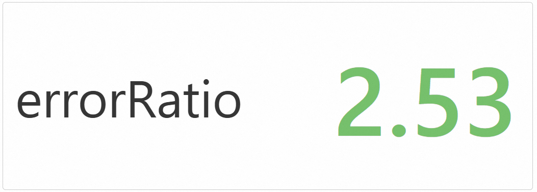
Example 9. Query the percentage for the number of error requests in NGINX logs

The number of error requests whose status code exceeds 400 and the total number of requests are obtained based on SQL statements. Then, the percentage for the number of error requests is calculated. The results are displayed in a statistical chart. (Demo)

• Query statement

  * |
  select
    round((errorCount * 100.0 / totalCount), 2) as errorRatio
  from
    (
      select
        sum(
          case
            when status >= 400 then 1
            else 0
          end
        ) as errorCount,
        count(1) as totalCount
      from
        log
    )

• Results