SPL functions - Simple Log Service - Alibaba Cloud Documentation Center

After you process time series data in a Logstore using Structured Process Language (SPL) instructions, call time series SPL functions to visualize the results.

Function list

Function name	Description
second_to_nano	A time conversion function. Converts second-level timestamps to nanosecond-level timestamps. This function is suitable for high-precision scenarios.
series_forecast	A time series prediction function. Predicts future trends based on historical data. This function is suitable for monitoring, analysis, and planning.
series_pattern_anomalies	An anomaly detection function. Uses machine learning algorithms to identify anomalous points or patterns in a time series. This function is suitable for scenarios such as monitoring, alerting, and data analytics.
series_decompose_anomalies	A time series decomposition and anomaly detection function. Uses a time series decomposition algorithm to split raw data into trend, seasonal, and residual components. It then analyzes the residual component using statistical methods to identify anomalous points. This function is suitable for scenarios such as real-time monitoring, root cause analysis, and data quality detection.
series_drilldown	A drill-down function for time series analysis. It allows for fine-grained analysis of data within a specific time period based on time-grouped statistics.
cluster	Supports quick group analysis of multiple time series or vector data. It can identify metric curves with similar shapes, detect abnormal patterns, or categorize data patterns.
series_describe	A function for time series analysis. This function analyzes a time series from multiple dimensions and returns the results. The results include whether the data is continuous, the status of missing data, whether the sequence is stable, whether the sequence has periodicity and the length of the period, and whether the sequence has a significant trend.
correlation	Calculates the similarity between two objects. The function provides the following features: 1. If both objects are single vectors, it returns the similarity between the two sequences. 2. If one object is a group of vectors and the other is a single vector, it returns the similarity between each vector in the group and the single vector. 3. If both objects are groups of vectors, it returns a matrix of the pairwise similarities between the two groups of vectors.

second_to_nano function

The second_to_nano function is a time conversion function that converts timestamps from seconds to nanoseconds. It is typically used to process time fields in logs, especially in scenarios that require high-precision timestamps.

Important

Precision: Ensure that your database and application support sufficient precision to handle nanosecond-level time data.
Data type: Select an appropriate data type, such as BIGINT, to store nanosecond-level data to prevent overflow or precision loss.

Syntax

second_to_nano(seconds)

Parameters

Parameter	Description
seconds	The timestamp in seconds. The value can be an integer or a floating-point number.

Return value

Returns the corresponding timestamp in nanoseconds as an integer.

Example

Count the number of different requests in different time periods at the nanosecond level.

Query and analysis statement

* | extend ts = second_to_nano(__time__)
| stats count=count(*) by ts,request_method

Output

series_forecast function

The series_forecast function is used for time series prediction. It uses machine learning algorithms to predict future data points based on historical time series data. This function is often used in scenarios such as monitoring, trend analysis, and capacity planning.

Limits

You must construct the data in the series format using make-series. The time unit must be in nanoseconds.
Each row must contain at least 31 data points.

Syntax

series_forecast(array(T) field, bigint periods)

series_forecast(array(T) field, bigint periods, varchar params)

Parameters

Parameter	Description
field	The metric column of the input time series.
periods	The number of data points that you want to predict.
params	Optional. The algorithm parameters in the JSON format.

Return value

row(
  time_series array(bigint),
  metric_series array(double),
  forecast_metric_series array(double),
  forecast_metric_upper_series array(double),
  forecast_metric_lower_series array(double),
  forecast_start_index bigint,
  forecast_length bigint,
  error_msg varchar)

Column name	Type	Description
time_series	array(bigint)	An array of nanosecond-level timestamps. It includes the timestamps of the input time period and the predicted time period.
metric_series	array(double)	A metric array that has the same length as time_series. The original input metric is modified (for example, NaN values are modified) and the predicted time period is extended with NaN values.
forecast_metric_series	array(double)	An array of prediction results that has the same length as time_series. It includes the fitted values of the input metric and the predicted values for the predicted time period.
forecast_metric_upper_series	array(double)	An array of the upper bounds of the prediction results. The length is the same as time_series.
forecast_metric_lower_series	array(double)	An array of the lower bounds of the prediction results. The length is the same as time_series.
forecast_start_index	bigint	The start index of the predicted time period in the timestamp array.
forecast_length	bigint	The number of data points in the predicted time period in the timestamp array.
error_msg	varchar	The error message. If the value is null, the time series prediction is successful. Otherwise, the value indicates the reason for the failure.

Example

Count the number of different request_method values for the next 10 data points.

SPL statement

* | extend ts = second_to_nano(__time__ - __time__ % 60)
  | stats latency_avg = max(cast(status as double)), inflow_avg = min(cast (status as double)) by ts, request_method
  | make-series   latency_avg  default = 'last',
                inflow_avg default = 'last'
                on ts 
                from 'min' to 'max'
                 step '1m' 
                by request_method
 | extend test=series_forecast(inflow_avg, 10)

Output

Algorithm parameters

Parameter	Description
"pred":"10min"	The interval between data points in the expected prediction result. The supported units are: `D daily frequency H hourly frequency T, min minutely frequency S secondly frequency`
"uncertainty_config": {"interval_width": 0.9999}	The value of uncertainty_config.interval_width must be in the range of (0, 1). A larger value indicates a wider range between the upper and lower bounds in the prediction result.
"seasonality_config": {"seasons": [{"name": "month", "period": 30.5, "fourier_order": 1}]}	The seasonality_config.seasons parameter contains custom time series periods. name: the name of the period. periods: the number of days in each period. fourier_order: the fitting strength of the period. The service provides default settings for daily, weekly, and yearly periods. To fit other periods, configure them in seasonality_config.seasons.

series_pattern_anomalies function

The series_pattern_anomalies function detects abnormal patterns in time series data. It uses machine learning algorithms to automatically identify anomalous points or patterns in a time series. This function is suitable for scenarios such as monitoring, alerting, and data analytics.

Limits

You must construct the data in the series format using make-series. The time unit must be in nanoseconds.
Each row must contain at least 11 data points.

Syntax

series_pattern_anomalies(array(T) metric_series)

Parameters

Parameter	Description
metric_series	The metric column of the input time series. Only numeric types are supported.

Return value

row(
  anomalies_score_series array(double),
  anomalies_type_series array(varchar)
  error_msg varchar
)

Column name	Type	Description
anomalies_score_series	array(double)	The anomaly score series, which corresponds to the input time series. The value is in the range of [0, 1] and represents the anomaly score of each data point.
anomalies_type_series	array(varchar)	The anomaly type description series, which corresponds to the input time series. It represents the anomaly type of each data point. Normal data points are represented as null.
error_msg	varchar	The error message. If the value is null, the time series anomaly detection is successful. Otherwise, the value indicates the reason for the failure.

Example

Detect anomalies in the sequence at the current data point.

SPL statement

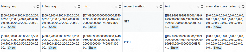
* | extend ts = second_to_nano(__time__ - __time__ % 60)
  | stats latency_avg = max(cast(status as double)), inflow_avg = min(cast (status as double)) by ts, request_method
  | where request_method is not null
  | make-series   latency_avg  default = 'last',
                inflow_avg default = 'last'
                on ts 
                from 'min' to 'max'
                 step '1m' 
                by request_method
 | extend test=series_pattern_anomalies(inflow_avg)

Output

series_decompose_anomalies function

The series_decompose_anomalies function is used for time series decomposition and anomaly detection. It uses a time series decomposition algorithm to split raw time series data into trend, seasonal, and residual components. It then detects anomalous points by analyzing the residual component.

Limits

You must construct the data in the series format using make-series. The time unit must be in nanoseconds.
Each row must contain at least 11 data points.

Syntax

series_decompose_anomalies(array(T) metric_series)

series_decompose_anomalies(array(T) metric_series, varchar params)

Parameters

Parameter	Description
metric_series	The metric column of the input time series.
params	Optional. The algorithm parameters in the JSON format.

Return value

row(
  metric_baseline_series array(double)
  anomalies_score_series array(double),
  anomalies_type_series array(varchar)
  error_msg varchar
)

Column name	Type	Description
metric_baseline_series	array(double)	The metric data that is fitted by the algorithm.
anomalies_score_series	array(double)	The anomaly score series, which corresponds to the input time series. The value is in the range of [0, 1] and represents the anomaly score of each data point.
anomalies_type_series	array(varchar)	The anomaly type description series, which corresponds to the input time series. It represents the anomaly type of each data point. Normal data points are represented as null.
error_msg	varchar	The error message. If the value is null, the time series anomaly detection is successful. Otherwise, the value indicates the reason for the failure.

Example

After performing anomaly detection on all time series, retain the time series from the last 5 minutes that have an anomaly score of 0 or higher.

SPL statement

* | extend ts = second_to_nano(__time__ - __time__ % 60)
  | stats latency_avg = max(cast(status as double)), inflow_avg = min(cast (status as double)) by ts, request_method
  | where request_method is not null
  | make-series   latency_avg  default = 'last',
                inflow_avg default = 'last'
                on ts 
                from 'min' to 'max'
                 step '1m' 
                by request_method
 | extend test=series_decompose_anomalies(inflow_avg, '{"confidence":"0.005"}')
 | extend anomalies_score_series = test.anomalies_score_series
 | where array_max(slice(anomalies_score_series, -5, 5)) >= 0

Output

Algorithm parameters

Parameter	Type	Example	Description
auto_period	varchar	"true"	Specifies whether to enable automatic detection of time series periods. Valid values: "true" and "false". If you set this parameter to "true", the custom period_num and period_unit parameters do not take effect.
period_num	varchar	"[1440]"	The number of data points that a sequence period contains. You can enter multiple period lengths. The service considers only the longest period.
period_unit	varchar	"[\"min\"]"	The time unit of each data point in the sequence period. You can enter multiple time units. The number of time units must be the same as the number of specified periods.
period_config	varchar	"{\"cpu_util\": {\"auto_period\":\"true\", \"period_num\":\"720\", \"period_unit\":\"min\"}}"	To set different periods for different features, configure the period_config field. In period_config, the field name is the name of the feature to be set, and the field value is an object in which you set the auto_period, period_num, and period_unit fields.
trend_sampling_step	varchar	"8"	The downsampling rate for the trend component during time series decomposition. The value must be a positive integer. A higher sample rate results in a faster fitting speed for the trend component, but reduces the fitting precision. Default value: "1".
season_sampling_step	varchar	"1"	The downsampling rate for the seasonal component during time series decomposition. The value must be a positive integer. A higher sample rate results in a faster fitting speed for the seasonal component, but reduces the fitting precision. Default value: "1".
batch_size	varchar	"2880"	Anomaly analysis uses a sliding window to process data in segments. batch_size specifies the size of the window. A smaller window size increases the analysis speed, but may decrease accuracy. By default, the window size is the same as the sequence length.
confidence	varchar	"0.005"	The sensitivity of anomaly analysis. The value must be a floating-point number in the range of (0, 1.0). A smaller value indicates that the algorithm is less sensitive to anomalies, which reduces the number of detected anomalies.
confidence_trend	varchar	"0.005"	The sensitivity to anomalies when the trend component is analyzed. If you set this parameter, the confidence parameter is ignored. A smaller value indicates that the algorithm is less sensitive to anomalies in the trend component, which reduces the number of detected anomalies in the trend component.
confidence_noise	varchar	"0.005"	The sensitivity to anomalies when the residual component is analyzed. If you set this parameter, the confidence parameter is ignored. A smaller value indicates that the algorithm is less sensitive to anomalies in the residual component, which reduces the number of detected anomalies in the residual component.

series_drilldown function

The series_drilldown function is a drill-down function for time series analysis. It allows for fine-grained analysis of data within a specific time period based on time-grouped statistics.

Syntax

series_drilldown(array(varchar) label_0_array,array(varchar) label_1_array,array(varchar) label_2_array, ... ,array(array(bigint)) time_series_array,array(array(double)) metric_series_array,bigint begin_time,bigint end_time)

series_drilldown(array(varchar) label_0_array,array(varchar) label_1_array,array(varchar) label_2_array, ... ,array(array(bigint)) time_series_array,array(array(double)) metric_series_array,bigint begin_time,bigint end_time,varchar config)

Parameters

Parameter	Description
label_x_array	Each element in the array is a label of the corresponding time series. The function overload supports a maximum of seven label arrays.
time_series_array	Each element in the outer array is a time series.
metric_sereis_array	Each element in the outer array is a metric series.
begin_time	The start time of the time range for which you want to perform a root cause drill-down. This is typically set to the start time of an anomaly. The unit is nanoseconds.
end_time	The end time of the time range for which you want to perform a root cause drill-down. This is typically set to the end time of an anomaly. The unit is nanoseconds.
config	Optional. The algorithm parameters in the JSON format.

Return value

row(dirlldown_result varchar, error_msg varchar)

Column name	Type	Description
dirlldown_result	varchar	The drill-down result in the JSON format.
error_msg	varchar	The error message. If the value is null, the time series prediction is successful. Otherwise, the value indicates the reason for the failure.

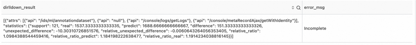
dirlldown_result parameter description

{
  "attrs": [
    {
      "api": "/ids/ml/annotationdataset",
      "resource": "test"
    },
    {
      "api": "/console/logs/getLogs"
    }
  ],
  "statistics": {
    "relative_ratio": 0.5003007763190033,
    "relative_ratio_predict": 1.0000575873881987,
    "unexpected_difference": -4.998402840764594,
    "relative_unexpected_difference": -0.499660063545782,
    "difference": -4.999183856137503,
    "predict": 5.005203022057271,
    "relative_ratio_real": 1.9987568734256989,
    "real": 10.004386878194774,
    "support": 50
  }
}

attrs parameter description

This parameter identifies the dimension filtering conditions that correspond to the statistical result. The conditions in the array are evaluated with an OR relationship.

In this example, api is /ids/ml/annotationdataset or /console/logs/getLogs.

  "attrs": [
    {
      "api": "/ids/ml/annotationdataset",
      "resource": "test"
    },
    {
      "api": "/console/logs/getLogs"
    }
  ]

In this example, the first element in attrs indicates that api is /ids/ml/annotationdataset and resource is test.
```
    {
      "api": "/ids/ml/annotationdataset",
      "resource": "test"
    }
```

statistics parameter description

This parameter provides the statistical analysis results of a time series for root cause analysis or anomaly detection.

Metric name	Type	Description
support	int	The statistical sample size, such as the number of data points, within the current root cause range.
real	float	The actual observed value of the metric within the current root cause range.
predict	float	The predicted value of the metric within the current root cause range.
difference	float	The absolute difference between the actual value and the predicted value of the metric within the current root cause range. Formula: predict - real.
unexpected_difference	float	The difference between the predicted value and the actual value after normal fluctuations (expected changes) are removed. This value indicates unexpected changes within the current root cause range.
relative_unexpected_difference	float	The ratio of unexpected changes to expected changes of the metric within the current root cause range.
relative_ratio	float	The ratio of the actual value to the baseline value of the metric within the current root cause range. Formula: predict / real.
relative_ratio_predict	float	The ratio of the predicted value of the metric within the current root cause range to the predicted value of the metric outside the root cause range.
relative_ratio_real	float	The ratio of the actual value of the metric within the current root cause range to the actual value of the metric outside the root cause range.

Example

SPL statement

*
| extend ts= (__time__- __time__%60)*1000000000
| stats access_count = count(1) by ts, Method, ProjectName
| extend access_count = cast( access_count as double)
| make-series   access_count = access_count default = 'null'
                on ts
                from 'sls_begin_time' to 'sls_end_time'
                step '1m'
                by Method, ProjectName
| stats m_arr = array_agg(Method), ProjectName = array_agg(ProjectName), ts_arr = array_agg(__ts__), metrics_arr = array_agg(access_count)
| extend ret = series_drilldown(ARRAY['Method', 'Project'], m_arr, ProjectName, ts_arr, metrics_arr, 1739192700000000000, 1739193000000000000, '{"fill_na": "1", "gap_size": "3"}')
| project ret

Output

cluster function

The cluster function supports quick group analysis of multiple time series or vector data. It can identify metric curves with similar shapes, detect abnormal patterns, or categorize data patterns.

Syntax

cluster(array(array(double)) array_vector, varchar cluster_mode,varchar params)

Parameters

Parameter	Description
array_vector	A two-dimensional vector. You must ensure that the vectors in each row have the same length.
cluster_mode	The clustering model. Simple Log Service provides two models: kmeans dbscan
params	The algorithm parameters vary based on the clustering model.

Clustering models

kmeans

{
  "n_clusters": "5",
  "max_iter": "100",
  "tol": "0.0001",
  "init_mode": "kmeans++",
  "metric": "cosine/euclidean"
}

The following list describes optimization methods and suggestions for adjusting the parameters of the k-means algorithm:

n_clusters (number of clusters): The current value is 5. Use the elbow method to select an appropriate number of clusters. Observe the trend of the sum of squared errors (SSE) and adjust the value to 3, 7, or another value based on the results.
max_iter (maximum number of iterations): The current value is 100. For large datasets, you may need to increase the number of iterations to ensure convergence. If the results stabilize early, reduce this value to conserve computing resources. The value is typically in the range of 100 to 300.
tol (convergence toleration): This parameter controls the convergence condition of the algorithm and defines the threshold for the change in cluster centers. For high-precision requirements, you can decrease the value to 0.00001. For large datasets, you can increase the value to 0.001 to improve efficiency. You must balance computing efficiency and precision.
init_mode (initialization mode): The current value is kmeans++, which typically provides good initial cluster centers. Try random initialization as needed, but it may require more iterations. If the initial cluster centers have a significant impact on the results, explore different initialization strategies.
metric (cosine/euclidean):
- cosine (cosine similarity): Calculates the cosine of the angle between vectors to measure similarity in direction. This metric is suitable for high-dimensional data, such as text embeddings and image feature vectors, and similarity matching tasks, such as recommendation systems. When data is normalized to unit vectors, cosine similarity is equivalent to the inner product.
- euclidean (Euclidean distance): Calculates the straight-line distance between two points to measure absolute distance differences. This metric is suitable for geometric problems in low-dimensional spaces, such as coordinate points, and distance-sensitive tasks, such as k-means clustering and k-nearest neighbors classification or regression. It is also suitable for scenarios where the absolute value differences in data must be preserved.

dbscan

{
  "epsilon": "0.1", // Note: If the value of epsilon is less than or equal to 0, the algorithm automatically infers this parameter.
  "min_samples": "5"
}

The Density-Based Spatial Clustering of Applications with Noise (DBSCAN) algorithm has two key parameters, epsilon (ε) and min_samples, which define the density criteria for clusters:

epsilon (ε): Defines the neighborhood range of a point to determine whether points are adjacent. A smaller ε value may result in more noise points, whereas a larger ε value may merge unrelated points. The appropriate ε value is typically selected by observing the elbow point in a k-distance graph.
min_samples: Defines the minimum number of points required to form a dense cluster. A higher value makes the algorithm stricter, which reduces the number of clusters and increases the number of noise points. A lower value may include less dense areas. The value is generally selected based on the data dimensionality. For example, you can set the value to 4 or 5 for two-dimensional data.

These two parameters together determine how clusters are formed and how noise points are identified. The advantage of DBSCAN is that it can identify clusters of arbitrary shapes without requiring you to specify the number of clusters. However, its performance is highly sensitive to parameter selection. You typically need to adjust the parameters based on experiments and data characteristics to achieve optimal clustering results.

Return value

row(
  n_clusters bigint, 
  cluster_sizes array(bigint), 
  assignments array(bigint),  
  error_msg varchar 
)

Column name	Type	Description
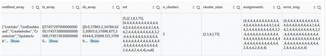
n_clusters	bigint	The number of clusters in the returned clustering result.
cluster_sizes	array(bigint)	The number of samples that each cluster center contains.
assignments	array(bigint)	The ID of the cluster to which each input sample belongs.
error_msg	varchar	The error message that is returned if the call fails.

Example

SPL statement

* and __tag__:__job__: sql-calculate-metric
| extend time = cast(time as bigint) - cast(time as bigint) % 300 
| extend time = second_to_nano(time) 
| stats avg_latency = avg(cast(sum_latency as double)) by time, Method 
| make-series avg_latency = avg_latency default = '0' on time from 'sls_begin_time' to 'sls_end_time' step '5m' by Method 
| stats method_array = array_agg(Method), ts_array = array_agg(__ts__), ds_array = array_agg(avg_latency)
| extend ret = cluster(ds_array, 'kmeans', '{"n_clusters":"5"}')
| extend n_clusters = ret.n_clusters, cluster_sizes = ret.cluster_sizes, assignments = ret.assignments, error_msg = ret.assignments

Output

series_describe function

The series_describe function is used for time series analysis. This function analyzes a time series from multiple dimensions and returns the results. The results indicate whether the data is continuous, the status of missing data, whether the sequence is stable, whether the sequence has periodicity and the length of the period, and whether the sequence has a significant trend.

Limits

You must construct the data in the series format using make-series. The time unit must be in nanoseconds.

Syntax

series_describe(__ts__ array<bigint>, __ds__ array<double>)

series_describe(__ts__ array<bigint>, __ds__ array<double>,config varchar)

Parameters

Parameter	Description
__ts__	A monotonically increasing time series that represents the Unix timestamp in nanoseconds of each data point in the time series.
__ds__	A numeric sequence of the floating-point number type. It represents the numeric values at the corresponding data points and has the same length as the time series.
config	Optional. The algorithm parameters. The following list describes the default parameters. You can also customize the parameters. `"with_period": "True"`: Specifies whether to enable period detection. True indicates that period detection is enabled. `"with_stable": "True"`: Specifies whether to enable stability detection. True indicates that stability detection is enabled. `"with_trend": "True"`: Specifies whether to enable trend detection for the sequence. True indicates that trend detection is enabled. Example: `series_describe(__ts__, __ds__, '{"with_period": "True"}')`

Return value

row(statistic varchar, error_msg varchar)

Column name	Type	Description
statistic	varchar	A JSON-serialized string that is used to save the statistical information of the sequence.
cluster_sizes	array(bigint)	The number of samples that each cluster center contains.

statistic example

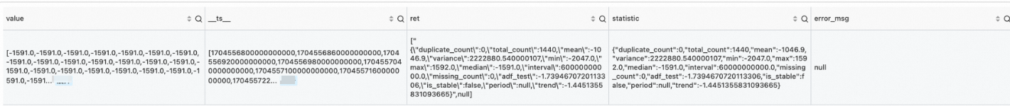
The returned result is a JSON-serialized string.

{
	"duplicate_count": 0, 
	"total_count": 1,
	"mean": 3.0,
	"variance": null,
	"min": 3.0,
	"max": 3.0,
	"median": 3.0,
	"interval": null,
	"missing_count": 0,
	"adf_test": null,
	"is_stable": false,
	"period": null,
	"trend": null
}

Parameter	Description
duplicate_count	The number of duplicate values.
total_count	The total number of data points.
mean	The average value.
variance	The variance. In this example, the value is `null`, which indicates that the variance is not calculated or applicable.
min	The minimum value.
max	The maximum value.
median	The median.
interval	The time interval. In this example, the value is `null`, which indicates that the interval is not calculated or applicable.
missing_count	The number of missing values.
adf_test	The result of the ADF test. In this example, the value is null, which indicates that the test is not performed or applicable.
is_stable	Indicates whether the data is stable. This is a Boolean value.
period	The period. In this example, the value is `null`, which indicates that no period is detected or the parameter is not applicable.
trend	The trend. In this example, the value is `null`, which indicates that no trend is detected or the parameter is not applicable.

Example

SPL statement

* and entity.file_name: "239_UCR_Anomaly_taichidbS0715Master.test.csv"
| extend time = cast(__time__ as bigint) 
| extend time = time - time % 60 
| stats value = avg(cast(value as double)) by time 
| extend time = second_to_nano(time)
| make-series value = value default = 'nan' on time from 'min' to 'max' step '1m' 
| extend ret = series_describe(value)

Output

correlation function

The correlation function calculates the similarity between two objects. The behavior of the function depends on the input:

Limits

The input parameters must be data in the series format that is constructed using make-series.

Syntax

Overload 1

correlation(arr_1 array(double), arr_2 array(double), params varchar)

Overload 2

correlation(arr_arr_1, array(array(double)), arr_2 array(double), params varchar)

Overload 3

correlation(arr_arr_1 array(array(double)), arr_arr_2  array(array(double)), params varchar)

Parameters

Overload 1

Parameter	Description
arr_1	A time series, which is a single unit generated by make-series.
arr_2	A time series, which is a single unit generated by make-series.
params	Optional. The algorithm parameters in the JSON format.

Overload 2

Parameter	Description
arr_arr_1	A time series, which is a single unit generated by make-series, is processed and returned as a two-dimensional array using the array_agg function.
arr_2	A time series, which is a single unit generated by make-series.
params	Optional. The algorithm parameters in the JSON format.

Overload 3

Parameter	Description
arr_arr_1	A time series, which is a single unit generated by make-series, is processed and returned as a two-dimensional array using the array_agg function.
arr_arr_2	A time series, which is a single unit generated by make-series, is processed and returned as a two-dimensional array using the array_agg function.
params	Optional. The algorithm parameters in the JSON format.

Algorithm parameters

Parameter name	Parameter explanation	Parameter type	Required
measurement	The method that is used to calculate the correlation coefficient. In most cases, you can use "Pearson". Valid values: Pearson: Pearson Correlation Coefficient. Measures the linear relationship between two continuous variables. SpearmanRank: Spearman's Rank Correlation Coefficient. Measures the monotonic relationship between two ordered variables to check whether their trends are consistent. KendallTau: Kendall's Tau Rank Correlation Coefficient. Measures the monotonic relationship between two ordered variables, with a focus on the consistency of their sorting. PointBiserial: Point-Biserial Correlation Coefficient. Measures the relationship between a binary categorical variable and a continuous variable.	varchar	Yes
max_shift	The maximum number of time series points that the first variable (the vector that corresponds to the first parameter) can be shifted to the left. A negative value indicates that the first variable can be shifted to the right. The output correlation coefficient is the maximum correlation coefficient when shifting is allowed.	integer	No. Default value: 0. A value of 0 indicates that shifting is not allowed.
flag_shift_both_direction	Valid values: true: The first variable can be shifted to the left or right by \|max_shift\| time series points. false: The first variable can be shifted only in the direction that is specified by the sign of max_shift.	boolean	No. Default value: "false".

Return value

Overload 1
```
row(result double)
```
Column name
Type
Description
result
double
The correlation coefficient between the input parameters arr_1 and arr_2.
Overload 2
```
row(result  array(double))
```
Column name
Type
Description
result
array(double)
An array of correlation coefficients between each vector in arr_arr_1 and arr_2. The length of the returned array is the number of vectors in arr_arr_1.
Overload 3
```
row(result  array(array(double)))
```
Column name
Type
Description
result
array(array(double))
A matrix. If the data is not empty, the element at row i and column j is the correlation coefficient between arr_arr_1[i] and arr_arr_2[j].

Examples

Example 1

SPL statement

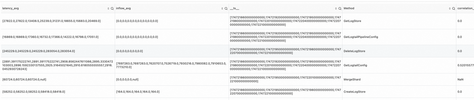
* | where Method != 'GetProjectQuery'
  | extend ts = second_to_nano(__time__ - __time__ % 60)
  | stats latency_avg = max(cast(avg_latency as double)), inflow_avg = min(cast (sum_inflow as double)) by ts, Method
  | make-series  latency_avg default = 'next',
                inflow_avg default = 'next'
                on ts
                from 'sls_begin_time' to 'sls_end_time'
                step '1m'
                by Method

  | extend correlation_scores = correlation( latency_avg, inflow_avg )

Output

Example 2

SPL statement

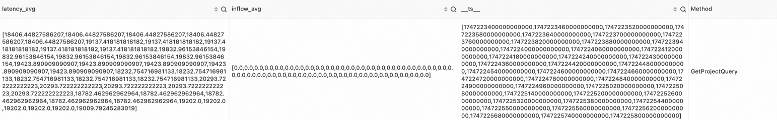
* | where Method='GetProjectQuery'
  | extend ts = second_to_nano(__time__ - __time__ % 60)
  | stats latency_avg = max(cast(avg_latency as double)), inflow_avg = min(cast (sum_inflow as double)) by ts, Method
  | make-series   latency_avg default = 'last',
                inflow_avg default = 'last'
                on ts
                from 'min' to 'max'
                step '1m'
                by Method
  | extend scores = correlation( latency_avg, inflow_avg, '{"measurement": "SpearmanRank", "max_shift": 4}' )

Output

Example 3

SPL statement

* | where Method='GetProjectQuery'
  | extend ts = second_to_nano(__time__ - __time__ % 60)
  | stats latency_avg = max(cast(avg_latency as double)), inflow_avg = min(cast (sum_inflow as double)) by ts, Method
  | make-series   latency_avg default = 'last',
                inflow_avg default = 'last'
                on ts
                from 'min' to 'max'
                step '1m'
                by Method
  | extend scores = correlation( latency_avg, inflow_avg, '{"measurement": "KendallTau", "max_shift": 5, "flag_shift_both_direction": true}')

Output