Simple Log Service:Data conversion

Types of data conversion rules

When you create a chart, you can configure data conversion rules. The supported types are Connect, Category, Parse Timestamp, Group By, and Transpose Rows and Columns.

• Category: groups the results of a query statement based on specified fields and performs calculation for each group. The following table describes the parameters. For more information, see Example for Category.

  Parameter	Description
  Select Data Source	Select the query statement whose results you want to classify. For example, if you select A, the results of Query Statement A are classified.
  X-axis	Select a field as the x-axis.
  Y-axis	Select a field as the y-axis.
  Aggregate Column	Select a field to further classify and aggregate data. For example, selecting the kind field classifies and aggregates data by that field.

• Connect: merges the results of multiple query statements by using Left Join, Right Join, or Full Join and displays the merged results in the chart. The following table describes the parameters. For more information, see Example for Connect.

  Parameter	Description
  Connection Mode	Select the join method for merging query results.
  Connection Field	Select a field common to all query results as the join key.

For example, for data conversion TA, set the type to Category, Select Data Source to A, x-axis to Time, y-axis to count, and aggregate column to kind. For data conversion TB, set the type to Connect, Connection Mode to Left Join, and Connection Field to Time.

Example for Connect

Query statements A and B both return results that include the time field. You can use Left Join on the time field to merge the results and display them in a table.

• Query and analysis configuration: Query and analysis A uses LogStore (SQL). The Logstore is sls-mall-traces and the statement is * | select __time__ - __time__ % 60 as time, count() as pv, 'computer' as icon, 'database' as database from log group by time order by time asc limit 2000. Query and analysis B uses LogStore (SQL). The Logstore is sls-mall-traces-deps and the statement is * | select __time__ - __time__ % 60 as time, count() as pvb from log group by time order by time asc limit 2000.

• Results of query and analysis A: The returned table contains four columns: time, pv, icon, and database. It shows statistical data grouped in 60-second intervals.

• Results of query and analysis B: The returned table contains two columns: time and pvb. It shows PVB statistical data grouped in 60-second intervals.

• Data conversion configuration: Set the type to Connect, Connection Mode to Left Join, and Connection Field to time.

• Data conversion results: After the Left Join, the combined table contains five columns: time, pvb, pv, icon, and database. The two result sets are merged based on the time field.

Example for Category

Query statement A aggregates data and groups it by the kind and time fields. A line chart displays only part of the results. To show all categories, configure a Category data conversion rule that classifies the results into five groups based on the kind field: producer, consumer, server, client, and internal. The line chart then displays the count for each category.

• Query and analysis configuration: Query and analysis A uses LogStore (SQL). The Logstore is sls-mall-traces and the statement is * | SELECT __time__ - __time__ % 60 AS Time, count(1) AS count, kind GROUP BY Time, kind ORDER BY Time LIMIT 1000.

• Query results before data conversion

  • Table: The returned table contains three columns, Time, count, and kind, with 80 rows in total. Each time point has a corresponding count for the five kind types: producer, consumer, server, client, and internal.

  • Line chart

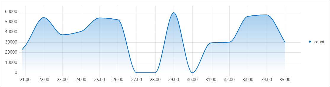
• Data conversion configuration: Set the type to Category, Select Data Source to A, x-axis to Time, y-axis to count, and aggregate column to kind.

• Query results after data conversion

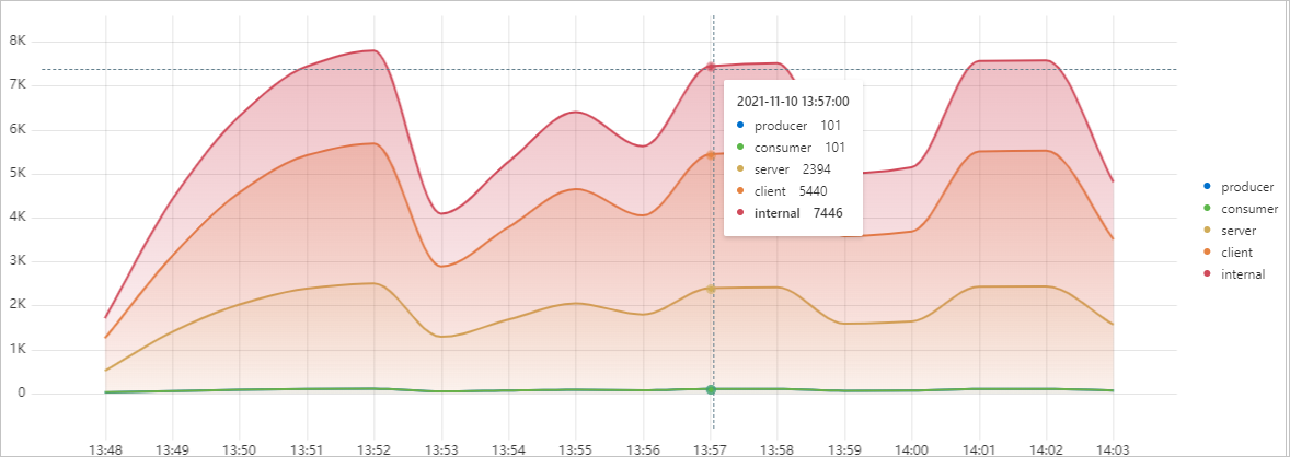
  • Table: The categorized table splits the data into five separate columns based on the kind field: consumer, producer, internal, server, and client. Each row displays the count for each category at the same time point.

  • Line chart

Example for Parse Timestamp

After query statement A returns results, you can configure a Parse Timestamp data conversion rule to parse a specific field into a UNIX timestamp.

• Query statement

  Query and analysis A uses Logstore (SQL). The query statement is * | select *.

• Results of Query Statement A

  The returned table includes columns such as __line__, file, info, time, __time__, and _source_. The time column contains values in the format 2024-03-04T10:31:27.427014. The result set has 82 rows.

• Data conversion configuration

  Set the data conversion type to Parse Timestamp, Select Data Source to A, field to time, and Format to YYYY-MM-DD HH:mm:ss.

• Data conversion results

  In the converted table, the values in the time column are parsed from a time string into a UNIX timestamp format (such as 1720578030). The table contains 82 rows.

Example for Group By

Query statements A and B both return results that include the request_method field. You can use Group By on this field to merge and aggregate the results in a table.

• Query statements

  Both query and analysis A and B use Logstore (SQL). The Logstore is nginx-access-log. The query statement for both is * | SELECT request_method, COUNT(*) as c group by request_method.

• Results of Query Statement A

  The result table for query and analysis A contains two columns, request_method and c, with counts for each method: HEAD(1), GET(237), DELETE(17), POST(62), and PUT(64).

• Results of Query Statement B

  The results for query and analysis B are identical to those of query and analysis A, containing the same request_method values and corresponding counts.

• Data conversion configuration

  Set the data conversion type to Group By, group by the request_method field, and apply the Sum function to the c field.

• Data conversion results

  The result after the Group By data conversion shows the combined statistics from both query and analysis operations: GET(474), POST(124), PUT(128), DELETE(34), and HEAD(2).

Example for Transpose Rows and Columns

After query statement A returns results, you can configure a Transpose Rows and Columns data conversion rule to swap the rows and columns.

• Query statement

  Query and analysis A uses Logstore (SQL). The query statement is * | select *.

• Results of Query Statement A

  The returned table includes columns such as __line__, file, info, time, __time__, and _source_. The time column contains values in the format 2024-03-04T10:31:27.427014. The result set has 82 rows.

• Data conversion configuration

  Set the data conversion type to Transpose Rows and Columns and select A as the data source.

• Data conversion results

  The new table has 82 columns (one for each original row) and a number of rows equal to the original column count. In the transposed table, the original rows become columns, and the original columns become rows.