Hierarchical Navigable Small World (HNSW) is the industry standard for high-performance, low-latency vector search. SelectDB has supported HNSW-based Approximate Nearest Neighbor (ANN) indexes since version 5.0. This topic explains how the HNSW algorithm works and how to create, query, and tune HNSW indexes in a SelectDB production cluster.
How it works
Background
The HNSW algorithm was introduced in the paper Efficient and robust approximate nearest neighbor search using Hierarchical Navigable Small World graphs (Malkov & Yashunin, 2016). To understand why HNSW is effective, it helps to understand the limitations of earlier approaches.
Proximity graph algorithms
Early approximate K-Nearest Neighbor (KNN) algorithms used proximity graphs, which approximate a Delaunay Graph. A Delaunay Graph has a key property: a greedy search always finds the nearest neighbor. These algorithms start from an entry point, then traverse the graph iteratively — at each step selecting the neighbor closest to the query vector — until no closer node is found.
Two problems limited these algorithms:
As data volume grows, the number of iterations scales according to a power law.
Building a high-quality proximity graph is difficult. Local clustering creates poorly connected regions where some nodes have almost no neighbors, making them hard to reach during search.
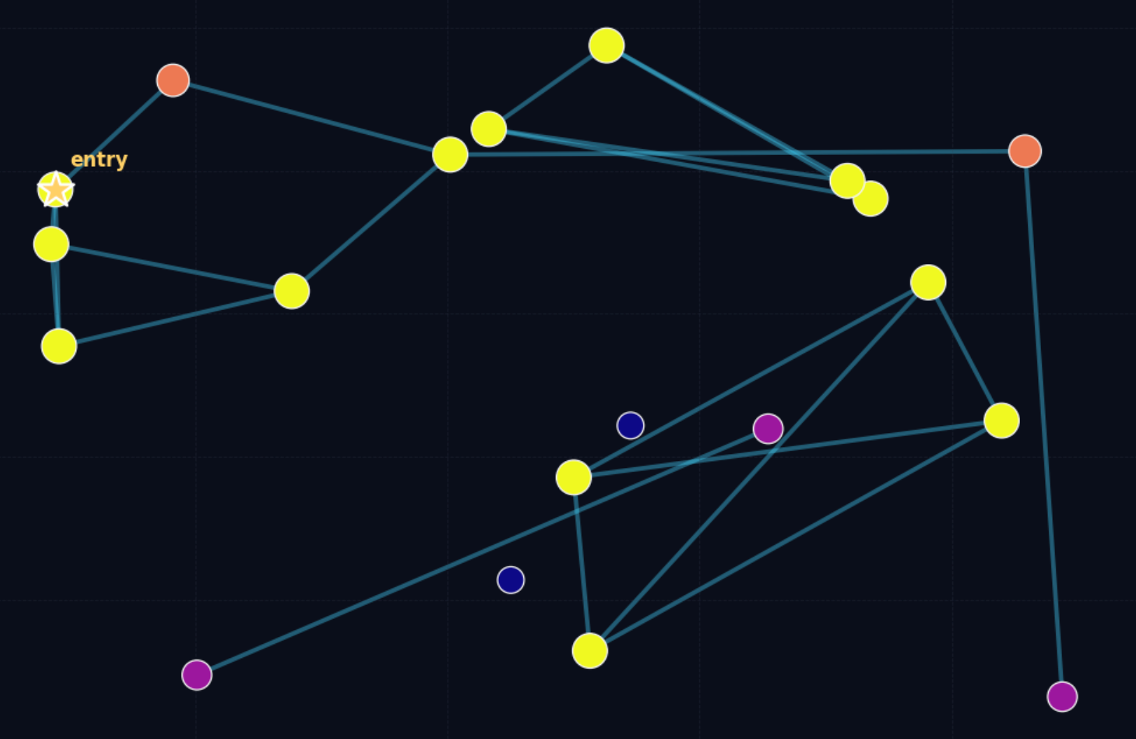
Navigable Small World (NSW)
Navigable Small World (NSW) addresses these problems by maintaining good connectivity while capping the maximum number of neighbors per node. This keeps search complexity logarithmic or polylogarithmic.
The NSW search has two phases:
Zoom-out: Start from a low-degree vertex and move toward higher-degree vertices until the average distance to neighbors exceeds the distance to the query vector.
Zoom-in: Once a high-degree vertex is found, run a greedy search to find the optimal Top-N results.
NSW's complexity is polylogarithmic because both the average number of hops and the average vertex degree have a logarithmic relationship with data size.
HNSW: hierarchical layers reduce complexity to logarithmic
HNSW reduces query time complexity from polylogarithmic to logarithmic by accelerating the zoom-out phase with a layered structure.
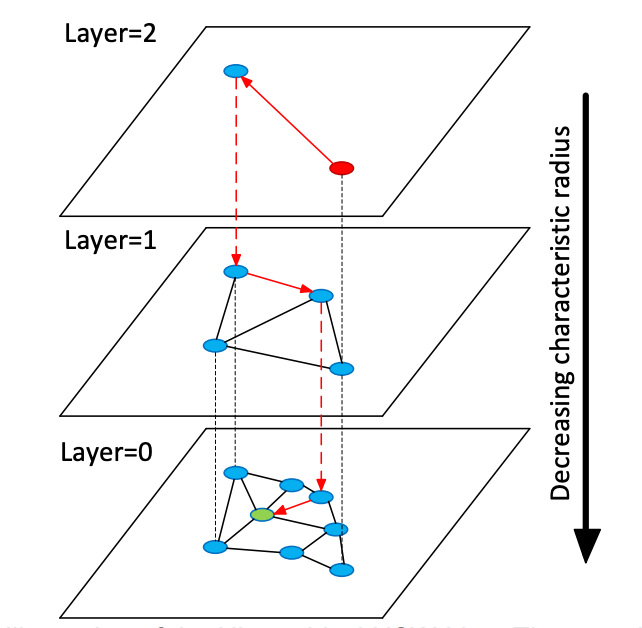
Each vector is assigned to one or more layers based on a geometric distribution. Higher layers are sparser and cover larger distances; lower layers are denser. Search starts at the top layer, performs a greedy search to find the nearest point, then descends to the next layer and repeats — all the way down to layer 0, where the fine-grained search produces the final results.
The maximum number of connections per node in each layer is capped by max_degree, which guarantees overall logarithmic time complexity.
Unlike NSW, HNSW does not require data to be shuffled before import. The random layer assignment during indexing acts as built-in randomization, which allows HNSW to support true incremental updates.
Create an HNSW index
SelectDB supports two methods for creating an HNSW index. Choose based on whether you are setting up a new table or adding an index to existing data.
| Method | When to use | Trade-offs |
|---|---|---|
| Inline index definition | New tables where data and index should be available together | Index is built on every import; compaction also triggers rebuilds, which increases resource usage |
| CREATE/BUILD INDEX | Large existing datasets; when you want to control when indexing happens | Import is faster; run full compaction before building the index to reduce write amplification |
Method 1: Define the index when creating a table
The index is built automatically each time data is imported. After import completes, the ANN index is immediately available for queries.
CREATE TABLE sift_1M (
  id int NOT NULL,
  embedding array<float> NOT NULL COMMENT "",
  INDEX ann_index (embedding) USING ANN PROPERTIES(
      "index_type"="hnsw",
      "metric_type"="l2_distance",
      "dim"="128"
  )
) ENGINE=OLAP
DUPLICATE KEY(id) COMMENT "OLAP"
DISTRIBUTED BY HASH(id) BUCKETS 1
PROPERTIES (
  "replication_num" = "1"
);

INSERT INTO sift_1M
SELECT *
FROM S3(
  "uri" = "https://selectdb-customers-tools-bj.oss-cn-beijing.aliyuncs.com/sift_database.tsv",
  "format" = "csv");
Method 2: Build the index after import
Create the table and import data without an index, then build the index separately. This approach is faster for large imports and gives you control over when index building happens.
Step 1: Create the table and import data.
CREATE TABLE sift_1M (
  id int NOT NULL,
  embedding array<float> NOT NULL COMMENT ""
) ENGINE=OLAP
DUPLICATE KEY(id) COMMENT "OLAP"
DISTRIBUTED BY HASH(id) BUCKETS 1
PROPERTIES (
  "replication_num" = "1"
);

INSERT INTO sift_1M
SELECT *
FROM S3(
  "uri" = "https://selectdb-customers-tools-bj.oss-cn-beijing.aliyuncs.com/sift_database.tsv",
  "format" = "csv");
Step 2: Run full compaction before building the index.
Building the index on fully merged segments produces a more stable recall rate and reduces write amplification from repeated index rebuilds during compaction.
Step 3: Define and build the index.
CREATE INDEX registers the index definition on the table but does not build it on existing data.
CREATE INDEX idx_test_ann ON sift_1M (`embedding`) USING ANN PROPERTIES (
  "index_type"="hnsw",
  "metric_type"="l2_distance",
  "dim"="128"
);
Verify that the index size is still 0 before building:
SHOW DATA ALL FROM sift_1M+-----------+-----------+--------------+----------+----------------+---------------+----------------+-----------------+----------------+-----------------+
| TableName | IndexName | ReplicaCount | RowCount | LocalTotalSize | LocalDataSize | LocalIndexSize | RemoteTotalSize | RemoteDataSize | RemoteIndexSize |
+-----------+-----------+--------------+----------+----------------+---------------+----------------+-----------------+----------------+-----------------+
| sift_1M | sift_1M | 1 | 1000000 | 170.001 MB | 170.001 MB | 0.000 | 0.000 | 0.000 | 0.000 |
| | Total | 1 | | 170.001 MB | 170.001 MB | 0.000 | 0.000 | 0.000 | 0.000 |
+-----------+-----------+--------------+----------+----------------+---------------+----------------+-----------------+----------------+-----------------+BUILD INDEX runs asynchronously and builds the index on all existing data:
BUILD INDEX idx_test_ann ON sift_1M;Monitor build progress:
SHOW BUILD INDEX WHERE TableName = "sift_1M"+---------------+-----------+---------------+------------------------------------------------------------------------------------------------------------------------------------+-------------------------+-------------------------+---------------+----------+------+----------+
| JobId | TableName | PartitionName | AlterInvertedIndexes | CreateTime | FinishTime | TransactionId | State | Msg | Progress |
+---------------+-----------+---------------+------------------------------------------------------------------------------------------------------------------------------------+-------------------------+-------------------------+---------------+----------+------+----------+
| 1763603913428 | sift_1M | sift_1M | [ADD INDEX idx_test_ann (`embedding`) USING ANN PROPERTIES("dim" = "128", "index_type" = "hnsw", "metric_type" = "l2_distance")], | 2025-11-20 11:14:55.253 | 2025-11-20 11:15:10.622 | 126128 | FINISHED | | NULL |
+---------------+-----------+---------------+------------------------------------------------------------------------------------------------------------------------------------+-------------------------+-------------------------+---------------+----------+------+----------+Drop an index
Drop an index when tuning hyperparameters, which requires testing different parameter combinations.
ALTER TABLE sift_1M DROP INDEX idx_test_ann;Run a vector query
High-dimensional vector strings add parsing overhead at query time. Avoid raw SQL for vector queries in high-concurrency production environments. Use the SelectDB vector search Python library instead — it uses prepared statements to parse SQL in advance, handles data conversion, and returns results directly as a pandas DataFrame.
from SelectDB_vector_search import SelectDBVectorClient, AuthOptions

auth = AuthOptions(
    host="localhost",
    query_port=9030,
    user="root",
    password="",
)

client = SelectDBVectorClient(database="demo", auth_options=auth)
tbl = client.open_table("sift_1M")

query = [0.1] * 128  # 128-dimensional query vector

# Equivalent SQL: SELECT id FROM sift_1M ORDER BY l2_distance_approximate(embedding, query) LIMIT 10;
result = tbl.search(query, metric_type="l2_distance").limit(10).select(["id"]).to_pandas()
print(result)
Output:
       id
0  123911
1   11743
2  108584
3  123739
4   73311
5  124746
6  620941
7  124493
8  177392
9  153178
Tune recall rate
Recall rate is the primary metric for vector search quality — all performance figures are meaningful only when the recall rate meets your target. Three factors affect recall rate:
Index and query hyperparameters (
max_degree,ef_construction,ef_search)Segment size and count
Vector quantization (covered in the vector quantization topic)
Understand the hyperparameters
All three parameters trade accuracy for speed or memory.
| Parameter | Phase | Effect | Trade-off |
|---|---|---|---|
max_degree | Build | Higher value → more edges per node → better recall | Increases memory usage and query latency |
ef_construction | Build | Higher value → more accurate neighbor search → better graph quality → better recall | Increases index build time |
ef_search | Query | Higher value → larger candidate set → better recall | Increases distance calculations and query latency |
SelectDB defaults: max_degree = 32, ef_construction = 40, ef_search = 32.
Build-phase internals
When a vector is inserted into the HNSW index:
Layer assignment: the vector is assigned to one or more layers using a geometric distribution — higher layers are sparser and serve as fast navigation shortcuts.
Candidate search: in each layer, HNSW runs a breadth-first local search using a candidate queue of length
ef_constructionto find the best neighbors.Connection limit: the number of neighbors is capped at
max_degreeto keep the graph structure bounded.
Query-phase internals
Coarse search: starting from the top layer, a greedy search descends layer by layer to quickly reach the target region.
Fine search: in layer 0, HNSW uses a candidate queue of length
ef_searchfor comprehensive neighborhood expansion.
Select hyperparameters
Different parameter combinations can achieve the same recall rate. The following table shows results from the SIFT 1M dataset (1 million 128-dimensional vectors) to illustrate the trade-off space.
| max_degree | ef_construction | ef_search | recall@1 | recall@100 |
|---|---|---|---|---|
| 32 | 80 | 32 | 0.955 | 0.75335 |
| 32 | 80 | 64 | 0.98 | 0.88015 |
| 32 | 80 | 96 | 0.995 | 0.9328 |
| 32 | 120 | 32 | 0.96 | 0.7736 |
| 32 | 120 | 64 | 0.975 | 0.89865 |
| 32 | 120 | 96 | 0.99 | 0.94575 |
| 32 | 160 | 32 | 0.955 | 0.78745 |
| 32 | 160 | 64 | 0.98 | 0.9097 |
| 32 | 160 | 96 | 0.995 | 0.95485 |
| 48 | 80 | 32 | 0.985 | 0.85895 |
| 48 | 80 | 64 | 0.99 | 0.9453 |
| 48 | 80 | 96 | 1 | 0.97325 |
| 48 | 120 | 32 | 0.97 | 0.78335 |
| 48 | 120 | 64 | 1 | 0.9089 |
| 48 | 120 | 96 | 1 | 0.95325 |
| 48 | 160 | 32 | 0.975 | 0.79745 |
| 48 | 160 | 64 | 0.995 | 0.9192 |
| 48 | 160 | 96 | 0.995 | 0.9601 |
| 64 | 80 | 32 | 1 | 0.9026 |
| 64 | 80 | 64 | 1 | 0.97025 |
| 64 | 80 | 96 | 1 | 0.9862 |
| 64 | 120 | 32 | 0.985 | 0.8548 |
| 64 | 120 | 64 | 0.99 | 0.94755 |
| 64 | 120 | 96 | 0.995 | 0.97645 |
| 64 | 160 | 32 | 0.97 | 0.80585 |
| 64 | 160 | 64 | 0.99 | 0.91925 |
| 64 | 160 | 96 | 0.995 | 0.96165 |
For a target recall@100 > 95%, any of these combinations work:
| max_degree | ef_construction | ef_search | recall@1 | recall@100 |
|---|---|---|---|---|
| 32 | 160 | 96 | 0.995 | 0.95485 |
| 48 | 80 | 96 | 1 | 0.97325 |
| 48 | 120 | 96 | 1 | 0.95325 |
| 48 | 160 | 96 | 0.995 | 0.9601 |
| 64 | 80 | 64 | 1 | 0.97025 |
| 64 | 80 | 96 | 1 | 0.9862 |
| 64 | 120 | 96 | 0.995 | 0.97645 |
| 64 | 160 | 96 | 0.995 | 0.96165 |
To find the optimal combination for your dataset, test multiple parameter combinations in parallel using a multi-index table:
Create a table named
table_multi_indexwith two or three vector fields but no indexes.Import data using Stream Load or another import method.
Create indexes on all vector fields using
CREATE INDEXandBUILD INDEX, with different parameters for each field.Measure recall rate on each field to identify the best combination.
Segment size and recall rate
SelectDB stores data in a hierarchical structure: table → tablets → rowsets → segments. Vector indexes operate at the segment level — each segment has its own HNSW index, and the recall rate depends on how many rows that segment covers.
A given set of hyperparameters has a limited effective data range. When a segment grows beyond a certain size, recall rate degrades. The following table provides empirical values for the SIFT 1M dataset:
| max_degree | ef_construction | ef_search | Segment rows | recall@100 |
|---|---|---|---|---|
| 32 | 160 | 96 | 1 million | 0.95485 |
| 48 | 80 | 96 | 1 million | 0.97325 |
| 32 | 160 | 32 | 3 million | 0.66983 |
| 128 | 512 | 128 | 3 million | 0.9931 |
Segment size is controlled by write_buffer_size and vertical_compaction_max_segment_size in the BE configuration. To check how many segments your table has, run SHOW TABLETS FROM table and follow the URL in the output.
Impact of compaction
Compaction can merge smaller segments into larger ones. If the resulting segments exceed the effective range of your current hyperparameters, recall rate drops. Run full compaction before BUILD INDEX — building on fully merged segments gives a more stable recall rate and reduces write amplification from repeated index rebuilds.
Query performance
Cold loading
SelectDB's ANN index is built on Faiss, Meta's open-source vector library. An HNSW index can accelerate queries only after its complete graph structure is loaded into memory. Before running high-concurrency queries, perform a cold query first to ensure that the index files for all relevant segments are loaded into memory. Skipping this step causes significantly higher latency until all files are loaded.
Memory planning
An HNSW index without quantization requires approximately 1.3x the raw memory size of the vectors it covers. Use this formula to estimate memory requirements:
Index memory ≈ num_vectors × dim × 4 bytes × 1.3Reference figures for common configurations:
| Dimensions | Rows | Estimated memory |
|---|---|---|
| 128 | 1 million | 650 MB |
| 768 | 10 million | 48 GB |
| 768 | 100 million | 110 GB |
If BE nodes run low on memory, the index is read from disk rather than memory, causing a sharp drop in query performance. Size your BE nodes to hold the full index in memory.
Reduce memory with quantization
Vector quantization compresses the index to reduce memory usage, at the cost of a small reduction in recall rate. Quantization options — including the trade-offs between memory savings and recall accuracy — are covered in the vector quantization topic.
What's next
Vector quantization: reduce memory usage with quantization compression