Optimize JOIN and Subquery Performance in Analytical Workloads - PolarDB for Xscale

PolarDB-X processes JOIN operations and subqueries at the computing layer, applying distributed JOIN algorithms and subquery optimization to minimize data movement and execution cost. This topic explains how the optimizer and executor handle each JOIN type and subquery pattern, and how to override the optimizer's decisions when needed.

Key concepts

JOIN operation — Combines rows from multiple tables based on one or more common columns. Semantically equivalent to computing the Cartesian product of two tables, then filtering the result. Most real-world JOINs are equi-joins (using equality conditions).

Subquery — A SELECT statement nested inside the WHERE or HAVING clause of an outer query. The result is passed to the outer query for further processing.

Execution scope — The JOIN operations described in this topic run at the computing layer. JOIN operations pushed down to LogicalView are executed by the MySQL engine at the storage layer.

JOIN types

PolarDB-X 1.0 supports the following JOIN types:

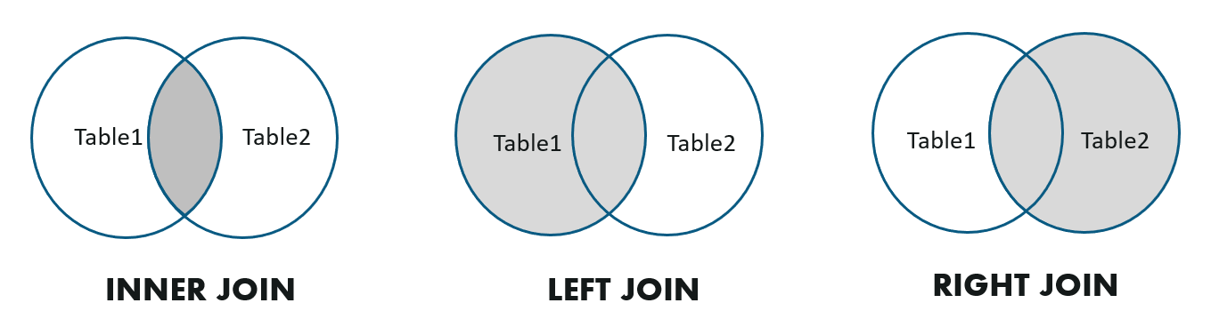
Common JOIN types — Written directly in SQL:

/* Inner join */
SELECT * FROM A, B WHERE A.key = B.key;

/* Left outer join */
SELECT * FROM A LEFT JOIN B ON A.key = B.key;

/* Right outer join */
SELECT * FROM A RIGHT OUTER JOIN B ON A.key = B.key;

Semi join and anti join — Cannot be expressed directly in SQL. PolarDB-X 1.0 implements them internally when it encounters subqueries with IN, NOT IN, EXISTS, or NOT EXISTS conditions:

/* Semi join — IN form */
SELECT * FROM Emp WHERE Emp.DeptName IN (
   SELECT DeptName FROM Dept
);

/* Semi join — EXISTS form */
SELECT * FROM Emp WHERE EXISTS (
  SELECT * FROM Dept WHERE Emp.DeptName = Dept.DeptName
);

/* Anti join — NOT IN form */
SELECT * FROM Emp WHERE Emp.DeptName NOT IN (
   SELECT DeptName FROM Dept
);

/* Anti join — NOT EXISTS form */
SELECT * FROM Emp WHERE NOT EXISTS (
  SELECT * FROM Dept WHERE Emp.DeptName = Dept.DeptName
);

JOIN algorithms

PolarDB-X 1.0 supports four distributed JOIN algorithms. The optimizer selects an algorithm based on cost estimates. Use a hint to override the optimizer's choice.

Algorithm selection

Algorithm	Best for	Requirement
Hash join	Large equi-joins where index lookup is not possible	Equality condition
Lookup join (BKA join)	Equi-joins where the outer table is small	Equality condition; inner table must be a single table
Sort-merge join	Equi-joins where the result must be sorted by the join key	Equality condition
Nested loop join	Non-equi joins, or when the inner table is very small	None

Nested loop join

Nested loop join is the general-purpose fallback algorithm, used for non-equi joins or when the inner table contains very little data. It is the least efficient algorithm for large datasets.

How it works:

Load all rows from the inner table (the right table, which typically has less data) into memory.
Scan the outer table row by row, comparing each row against the cached inner table.
Return rows that satisfy the join condition.

Example:

EXPLAIN SELECT * FROM partsupp, supplier WHERE ps_suppkey < s_suppkey;

NlJoin(condition="ps_suppkey < s_suppkey", type="inner")
  Gather(concurrent=true)
    LogicalView(tables="partsupp_[0-7]", shardCount=8, sql="SELECT * FROM `partsupp` AS `partsupp`")
  Gather(concurrent=true)
    LogicalView(tables="supplier_[0-7]", shardCount=8, sql="SELECT * FROM `supplier` AS `supplier`")

The < condition makes this a non-equi join, so the optimizer uses nested loop join.

Force nested loop join:

/*+TDDL:NL_JOIN(outer_table, inner_table)*/ SELECT ...

To specify multi-table groups as the inner or outer side:

/*+TDDL:NL_JOIN((outer_table_a, outer_table_b), (inner_table_c, inner_table_d))*/ SELECT ...

Hash join

Hash join is the most commonly used algorithm for equi-joins on large datasets, particularly when full table scans are unavoidable and index lookup is not applicable.

How it works:

Load all rows from the inner table (the right table, which typically has less data) into a hash table in memory. This is the build phase.
Scan the outer table row by row. For each outer row, probe the hash table using the join key to find matching rows.
Return rows that satisfy the join condition.

The inner (build) table is loaded into memory, so keep the smaller table on the inner side. The optimizer handles this automatically in most cases.

Example:

EXPLAIN SELECT * FROM partsupp, supplier WHERE ps_suppkey = s_suppkey;

HashJoin(condition="ps_suppkey = s_suppkey", type="inner")
  Gather(concurrent=true)
    LogicalView(tables="partsupp_[0-7]", shardCount=8, sql="SELECT * FROM `partsupp` AS `partsupp`")
  Gather(concurrent=true)
    LogicalView(tables="supplier_[0-7]", shardCount=8, sql="SELECT * FROM `supplier` AS `supplier`")

Both partsupp and supplier require full table scans, which makes hash join the right choice here.

Force hash join and specify join order:

/*+TDDL:HASH_JOIN(table_outer, table_inner)*/ SELECT ...

Lookup join (BKA join)

Lookup join (also known as BKA join, short for Batched Key Access join) is an equi-join algorithm suited for scenarios where the outer table has a small number of rows, allowing the inner table query to use index lookup efficiently.

Note

The inner table must be a single table. Lookup join cannot be used when the inner side is the result of joining multiple tables.

How it works:

Scan the outer table (the left table, which typically has less data) in batches (for example, every 1,000 rows).
For each batch, construct an IN (...) condition using the join keys of the batch.
Run the inner table query with that condition to retrieve matching rows.
Map the results back to outer rows using a hash table and return the merged result.

Example:

EXPLAIN SELECT * FROM partsupp, supplier WHERE ps_suppkey = s_suppkey AND ps_partkey = 123;

BKAJoin(condition="ps_suppkey = s_suppkey", type="inner")
  LogicalView(tables="partsupp_3", sql="SELECT * FROM `partsupp` AS `partsupp` WHERE (`ps_partkey` = ?)")
  Gather(concurrent=true)
    LogicalView(tables="supplier_[0-7]", shardCount=8, sql="SELECT * FROM `supplier` AS `supplier` WHERE (`s_suppkey` IN ('?'))")

The filter ps_partkey = 123 limits partsupp to a small number of rows. The generated s_suppkey IN (...) condition uses the primary key index on supplier, keeping the lookup cost low.

Force lookup join and specify join order:

/*+TDDL:BKA_JOIN(table_outer, table_inner)*/ SELECT ...

Sort-merge join

Sort-merge join is an equi-join algorithm that requires both input sides to be sorted on the join key before merging. It is not the most efficient algorithm in general, but becomes optimal when the query result must be ordered by the join key.

How it works:

Sort the rows from both input sides by the join key using MergeSort or MemSort.
Merge the sorted streams: advance the pointer on whichever side has the smaller current join key, and emit a result row when both sides match on the join key.

Example:

EXPLAIN SELECT * FROM partsupp, supplier WHERE ps_suppkey = s_suppkey ORDER BY s_suppkey;

SortMergeJoin(condition="ps_suppkey = s_suppkey", type="inner")
  MergeSort(sort="ps_suppkey ASC")
    LogicalView(tables="QIMU_0000_GROUP,QIMU_0001_GROUP.partsupp_[0-7]", shardCount=8, sql="SELECT * FROM `partsupp` AS `partsupp` ORDER BY `ps_suppkey`")
  MergeSort(sort="s_suppkey ASC")
    LogicalView(tables="QIMU_0000_GROUP,QIMU_0001_GROUP.supplier_[0-7]", shardCount=8, sql="SELECT * FROM `supplier` AS `supplier` ORDER BY `s_suppkey`")

Because the query includes ORDER BY s_suppkey, the optimizer chooses sort-merge join: the sort required by the algorithm also satisfies the output ordering, so no additional sort step is needed.

Force sort-merge join:

/*+TDDL:SORT_MERGE_JOIN(table_a, table_b)*/ SELECT ...

JOIN order

When joining N tables, the order in which the optimizer joins them affects the size of intermediate result sets and the overall execution cost.

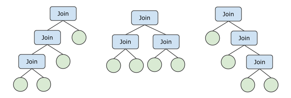
For a 4-table join that is not pushed down, the tables can be arranged in up to 24 (4!) orderings, and three different tree shapes (bushy, zig-zag, left-deep) are applicable — yielding up to 72 distinct join orders.

PolarDB-X 1.0 uses an adaptive strategy based on N:

N	Strategy	Reason
Small	Bushy tree — enumerates all orderings	Finds the optimal plan
Large	Zig-zag or left-deep tree	Reduces enumeration cost

The cost-based optimizer (CBO) selects the join order with the lowest estimated cost. For more information, see Introduction to the query optimizer.

Different algorithms also prefer different table positions. In a hash join, the inner (right) side builds the hash table, so the smaller table should be on the inner side. The CBO accounts for these preferences automatically.

Subqueries

PolarDB-X 1.0 supports most SQL subqueries. For the full list of supported syntax, see SQL limits.

Non-correlated vs. correlated subqueries

Type	Behavior	Execution
Non-correlated	Result does not depend on any outer column	Executed once in most cases
Correlated	References one or more columns from the outer query	Re-evaluated for each outer row

Examples:

/* Non-correlated: l_partkey IN (...) does not reference any outer column */
SELECT * FROM lineitem WHERE l_partkey IN (SELECT p_partkey FROM part);

/* Correlated: ps_suppkey = l_suppkey references the outer column l_suppkey */
SELECT * FROM lineitem WHERE l_partkey IN (SELECT ps_partkey FROM partsupp WHERE ps_suppkey = l_suppkey);

Subquery unnesting

PolarDB-X 1.0 converts compatible subqueries into semi join or JOIN operations — a process called unnesting. Unnesting eliminates repeated nested execution for each outer row, significantly reducing cost on large datasets.

Example — unnesting succeeds:

EXPLAIN SELECT p_partkey, (
      SELECT COUNT(ps_partkey) FROM partsupp WHERE ps_suppkey = p_partkey
      ) supplier_count FROM part;

Project(p_partkey="p_partkey", supplier_count="CASE(IS NULL($10), 0, $9)", cor=[$cor0])
  HashJoin(condition="p_partkey = ps_suppkey", type="left")
    Gather(concurrent=true)
      LogicalView(tables="part_[0-7]", shardCount=8, sql="SELECT * FROM `part` AS `part`")
    Project(count(ps_partkey)="count(ps_partkey)", ps_suppkey="ps_suppkey", count(ps_partkey)2="count(ps_partkey)")
      HashAgg(group="ps_suppkey", count(ps_partkey)="SUM(count(ps_partkey))")
        Gather(concurrent=true)
          LogicalView(tables="partsupp_[0-7]", shardCount=8, sql="SELECT `ps_suppkey`, COUNT(`ps_partkey`) AS `count(ps_partkey)` FROM `partsupp` AS `partsupp` GROUP BY `ps_suppkey`")

The correlated subquery is rewritten as a left hash join — the subquery no longer runs once per outer row.

When unnesting fails

Some subqueries cannot be unnested. In these cases, PolarDB-X 1.0 falls back to nested iteration: the subquery runs once for each row in the outer query. When the outer dataset is large, this can be slow.

Example — unnesting fails:

EXPLAIN SELECT * FROM lineitem WHERE l_partkey IN (SELECT ps_partkey FROM partsupp WHERE ps_suppkey = l_suppkey) OR l_partkey IS NOT NULL

Filter(condition="IS(in,[$1])[29612489] OR l_partkey < ?0")
  Gather(concurrent=true)
    LogicalView(tables="QIMU_0000_GROUP,QIMU_0001_GROUP.lineitem_[0-7]", shardCount=8, sql="SELECT * FROM `lineitem` AS `lineitem`")

>> individual correlate subquery : 29612489
Gather(concurrent=true)
  LogicalView(tables="QIMU_0000_GROUP,QIMU_0001_GROUP.partsupp_[0-7]", shardCount=8, sql="SELECT * FROM (SELECT `ps_partkey` FROM `partsupp` AS `partsupp` WHERE (`ps_suppkey` = `l_suppkey`)) AS `t0` WHERE (((`l_partkey` = `ps_partkey`) OR (`l_partkey` IS NULL)) OR (`ps_partkey` IS NULL))")

The OR condition prevents unnesting, leaving a correlated subquery that runs once per lineitem row. To fix this, remove the OR condition and rewrite the SQL to allow unnesting.

PolarDB:Optimize and execute JOIN operations and subqueries

Key concepts

JOIN types

JOIN algorithms

Algorithm selection

Nested loop join

Hash join

Lookup join (BKA join)

Sort-merge join

JOIN order

Subqueries

Non-correlated vs. correlated subqueries

Subquery unnesting

When unnesting fails

What's next