GanosBase Raster is a spatio-temporal engine extension for PolarDB for PostgreSQL that stores, manages, and analyzes raster data entirely within the database. This tutorial walks through a complete areal precipitation analysis workflow: importing discrete observation point data via FDW (Foreign Data Wrapper), running spatial interpolation to build a raster, generating contour lines and filled surfaces, computing zonal statistics, and calculating a final weighted areal precipitation value for any polygon boundary.
By the end of this tutorial, you will have:
Imported point and polygon shapefiles from OSS into PolarDB using
ganos_fdwProduced an IDW (Inverse Distance Weighting) interpolated raster from 36 observation points
Clipped the raster to an administrative boundary polygon
Generated contour lines and filled polygon surfaces at a 1-unit interval
Computed per-interval precipitation statistics using
ST_StatisticsCalculated a pixel-level area-weighted areal precipitation value
Key concepts
Raster data
Raster data divides real-world space into a grid of cells. Each cell, also called a pixel, holds a value that represents a property of that location — for example, precipitation, elevation, or signal strength.
Raster data falls into two categories:
Thematic data: Each pixel holds a measured or classified value, such as DEM (digital elevation model) data, pollutant concentration, signal strength, precipitation, land ownership, or vegetation type.
Image data (remote sensing imagery): Images captured by ground-based, aerial, or satellite platforms that reflect the electromagnetic characteristics of surface objects.
Because raster data carries both spatial and temporal attributes, it is also referred to as spatio-temporal raster data. Temporal attributes let you manage raster data as time series.
GanosBase Raster
GanosBase Raster is provided by PolarDB for PostgreSQL. It supports integration and analysis of raster data from remote sensing, photogrammetry, and thematic mapping sources. It also provides a GeoServer extension for publishing raster objects as OGC (Open Geospatial Consortium) services such as WMS (Web Map Service) or WMTS (Web Map Tile Service). GanosBase Raster can be used in a wide range of sectors, including meteorology, environmental monitoring, geological exploration, natural resource management, national defense, emergency response, telecommunications, media, transportation, urban planning, and homeland security.
Data model
A GanosBase raster dataset is organized as follows:
Raster: A raster dataset — for example, a remote sensing image or a TIFF file.
Tile: The basic storage unit of a raster object. Each tile is 256 × 256 pixels by default.
Band: A single 2D layer in a raster dataset. Each band consists of multiple tiles, each with its own coordinate numbers.
Cell: A pixel in a tile. Cells support multiple data types, including byte, short, int, and double.
Pyramid: A series of reduced-resolution versions of a raster used to speed up display. Level 0 is the original data; each higher level is a coarser resolution.
Metadata: Raster metadata including spatial extent, projection type, and pixel type.

In the database, a raster image is stored as a raster object. Each raster object is logically divided into bands, each holding the raw image data from the import process. Storage and management happen at the tile level. Tile size defaults to 256 × 256 pixels but can be changed. Each tile contains one or more bands, which in turn consist of cells representing pixels. Each raster object has its own metadata — spatial extent, data type, projection information, and coordinate numbers. If a raster is organized as a pyramid, each band has its own pyramid levels.
Advantages
GanosBase Raster uses an object-oriented storage structure: each raster — whether a remote sensing image or a DEM file — is stored as a single database record with a one-to-one mapping. Each record can hold a raster up to 1 TB. Direct operations on tiles are not permitted, which protects metadata integrity. The extension also integrates natively with time series data.
For storage efficiency, raster metadata is kept in the database while raster attribute data is stored on OSS (Object Storage Service), a low-cost object storage backend. This architecture makes large-scale raster analysis — such as processing thousands of images — practical at significantly lower storage costs.
Beyond standard spatial operations, GanosBase Raster provides statistical and algebraic operators, image color-balancing algorithms, and accelerated overview map rendering, all optimized for large-scale raster datasets.
Areal precipitation analysis
Background
Areal precipitation is a key indicator in flood forecasting. It represents the average precipitation per unit area within a region and provides critical data for flood control, reservoir management, disaster prevention, and economic planning. Monitoring networks collect data from isolated observation sites, so a computational pipeline is needed to produce region-wide areal precipitation estimates for decision-making.
How it works
This tutorial uses the following pipeline:
Import data: Load observation point data (shapefile) and administrative boundary data (shapefile) into the database using the GanosBase FDW extension.
Spatial interpolation: Use
ST_InterpolateRasterto convert discrete point observations into a continuous raster using the IDW method.Clip to boundary: Use
ST_ClipToRastto clip the interpolated raster to the administrative polygon boundary.Contour and surface generation: Use
ST_Contourto generate contour lines or filled polygon surfaces from the raster.Zonal statistics: Use
ST_Statisticsto compute precipitation statistics within any polygon area, broken down by value intervals.Areal precipitation: Traverse each pixel of the clipped raster, compute the area-weighted precipitation, and divide by the total area.
Prerequisites
Before you begin, ensure that you have:
A PolarDB for PostgreSQL instance
AccessKey ID and AccessKey Secret for an OSS bucket containing your shapefiles
Point shapefile (
point.shp) with ID (string) and precipitation (floating-point) attributesPolygon shapefile (
polygon.shp) representing the administrative boundary
Install the GanosBase extension
Install the ganos_raster and ganos_fdw extensions in your target database:
CREATE EXTENSION ganos_raster CASCADE;
CREATE EXTENSION ganos_fdw CASCADE;
Import data
Prepare a point layer file (
point.shp) and a polygon layer file (polygon.shp), both in ESRI Shapefile format. Each point has an ID attribute (string) and a precipitation attribute (floating-point). The following image shows the layers overlaid in QGIS, where each number is the precipitation value at that observation point: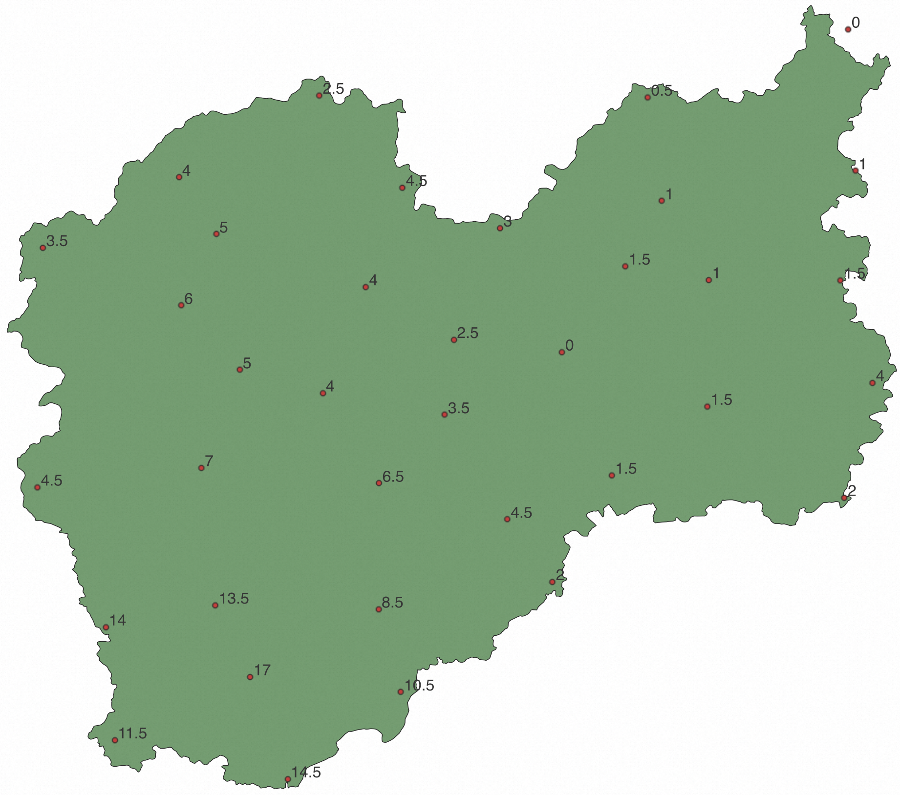
Map the shapefiles as foreign tables from OSS to the database using the GanosBase FDW, then create local tables and insert the data. Replace the placeholders in the following SQL with your actual OSS credentials and bucket path:
Placeholder Description Example <access_id>AccessKey ID LTAI5tXxx<secrect_key>AccessKey Secret xXxXxXxXx<Endpoint>OSS endpoint oss-cn-hangzhou.aliyuncs.com<bucket>OSS bucket name my-bucket<ak>AccessKey ID for user mapping LTAI5tXxx<ak_secret>AccessKey Secret for user mapping xXxXxXxXx-- ak and ak_secret are the AccessKeyId and AccessKeySecret of the OSS service. CREATE SERVER myserver FOREIGN DATA WRAPPER ganos_fdw OPTIONS ( datasource 'OSS://<access_id>:<secrect_key>@<Endpoint>/<bucket>/path_to/file', format 'ESRI Shapefile' ); CREATE USER MAPPING FOR CURRENT_USER SERVER myserver OPTIONS (user '<ak>', password '<ak_secret>'); -- Map shapefiles as external tables CREATE FOREIGN TABLE foreign_point_table ( fid integer, id varchar, geom geometry, pre double precision -- precipitation) SERVER myserver OPTIONS ( layer 'point' ); CREATE FOREIGN TABLE foreign_polygon_table ( fid integer, id varchar, geom geometry) SERVER myserver OPTIONS ( layer 'polygon' ); -- Create tables and insert data CREATE TABLE point_table AS SELECT fid, geom, pre FROM foreign_point_table; CREATE TABLE polygon_table AS SELECT fid, geom FROM foreign_polygon_table;Verify the import by querying
point_table:SELECT fid, ST_AsText(geom), pre FROM point_table;Expected output:
fid  |          st_astext          | pre
-----+-----------------------------+------
   0 | POINT(119.1084 28.50302)    |    5
   1 | POINT(118.768925 28.475747) |  3.5
   2 | POINT(119.30954 28.773729)  |  2.5
   3 | POINT(119.039694 28.363413) |    6
   4 | POINT(119.035561 28.614094) |    4
   5 | POINT(119.9517 28.77)       |  0.5
   6 | POINT(120.35833 28.62694)   |    1
   7 | POINT(119.908078 28.439481) |  1.5
   8 | POINT(119.472 28.5933)      |  4.5
   9 | POINT(119.400282 28.398895) |    4
  10 | POINT(119.783954 28.271403) |    0
  11 | POINT(119.663102 28.514025) |    3
  12 | POINT(120.343889 28.9031)   |    0
  13 | POINT(119.425841 27.768324) |  8.5
  14 | POINT(119.426237 28.015453) |  6.5
  15 | POINT(119.677214 27.944789) |  4.5
  16 | POINT(119.078999 28.045044) |    7
  17 | POINT(120.328711 28.411951) |  1.5
  18 | POINT(120.071226 28.412596) |    1
  19 | POINT(120.336292 27.986628) |    2
  20 | POINT(119.174307 27.635898) |   17
  21 | POINT(119.106197 27.776089) | 13.5
  22 | POINT(119.316833 28.191166) |    4
  23 | POINT(119.554612 28.149524) |  3.5
  24 | POINT(119.573099 28.295702) |  2.5
  25 | POINT(119.154161 28.237417) |    5
  26 | POINT(120.391447 28.211369) |    4
  27 | POINT(119.979144 28.568005) |    1
  28 | POINT(119.468737 27.606996) | 10.5
  29 | POINT(119.881658 28.03036)  |  1.5
  30 | POINT(120.068508 28.165111) |  1.5
  31 | POINT(119.765358 27.821914) |    2
  32 | POINT(118.892389 27.733222) |   14
  33 | POINT(118.75833 28.00694)   |  4.5
  34 | POINT(118.91 27.51222)      | 11.5
  35 | POINT(119.248086 27.435982) | 14.5
(36 rows)
Perform spatial interpolation
ST_InterpolateRaster converts point observations into a raster object using IDW interpolation. It supports parallel processing to improve performance on large datasets.
Create a table with a raster field to store the interpolated output:
CREATE TABLE IF NOT EXISTS raster_table
(
  id integer,
  rast raster -- raster data type for storing interpolated raster objects
);
Run
ST_InterpolateRasteronpoint_tableusing IDW and insert the result intoraster_table. The JSON options control the interpolation behavior: Thechunktableoption in the second JSON argument names the internal chunk storage table used by GanosBase.ST_MakePointis used here to create a 3D point geometry where the Z coordinate carries the precipitation value. This letsST_InterpolateRasterread precipitation as the attribute to interpolate.Key Description Example value methodInterpolation algorithm "IDW"radiusSearch radius in degrees. Larger values include more distant points and produce smoother output. 2.0max_pointsMaximum number of neighboring points to use. "30"min_pointsMinimum number of neighboring points required to produce a value. "1"INSERT INTO raster_table(id, rast) VALUES( 1, (SELECT ST_InterpolateRaster( ST_Collect(ST_MakePoint(ST_X(geom),ST_Y(geom),pre)), 512, 512, '{"method":"IDW","radius":2.0,"max_points":"30","min_points":"1"}', '{"chunktable":"rbt","celltype":"32bf"}') FROM point_table));For large point datasets, enable parallel processing before running the interpolation:
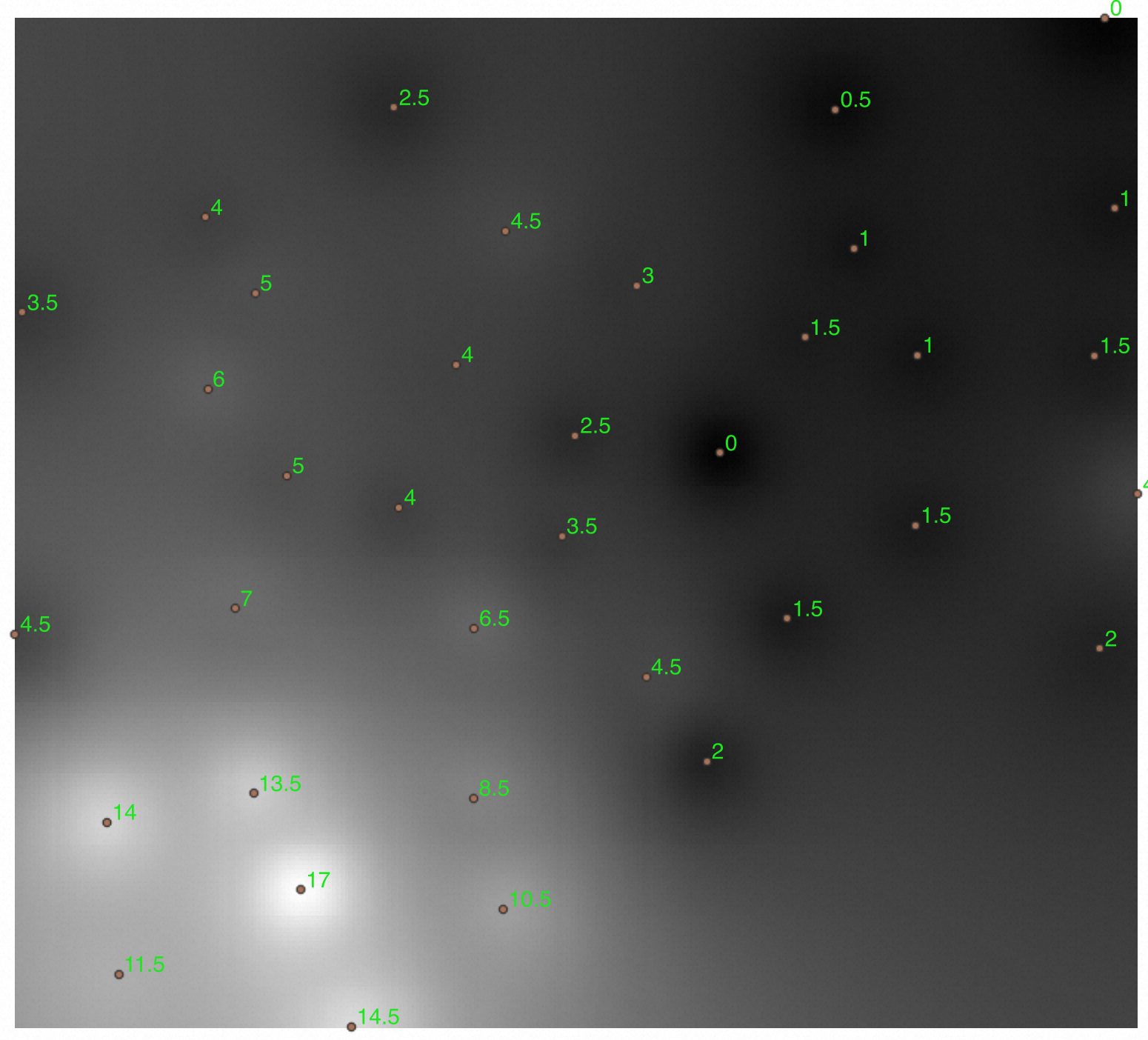
-- Set the degree of parallelism to 4
SET ganos.parallel.degree = 4;
Export the interpolated raster to a COG (Cloud Optimized GeoTIFF) file on OSS for inspection in QGIS:
SELECT ST_ExportTo(rast,
  'COG',
  'OSS://<access_id>:<secrect_key>@<Endpoint>/<bucket>/path_to/file.tif')
  FROM raster_table WHERE id=1;
The following image shows the interpolated raster opened in QGIS:
Clip the interpolated raster to the administrative boundary polygon from
polygon_tableand store the result asid=2:INSERT INTO raster_table SELECT 2, ST_ClipToRast(r.rast, p.geom, 0, '', NULL, '', '{"chunktable":"rbt"}') FROM raster_table AS R, polygon_table AS p;Export the clipped raster for verification:
SELECT ST_ExportTo(rast,
  'COG',
  'OSS://<access_id>:<secrect_key>@<Endpoint>/<bucket>/path_to/file.tif')
  FROM raster_table WHERE id=2;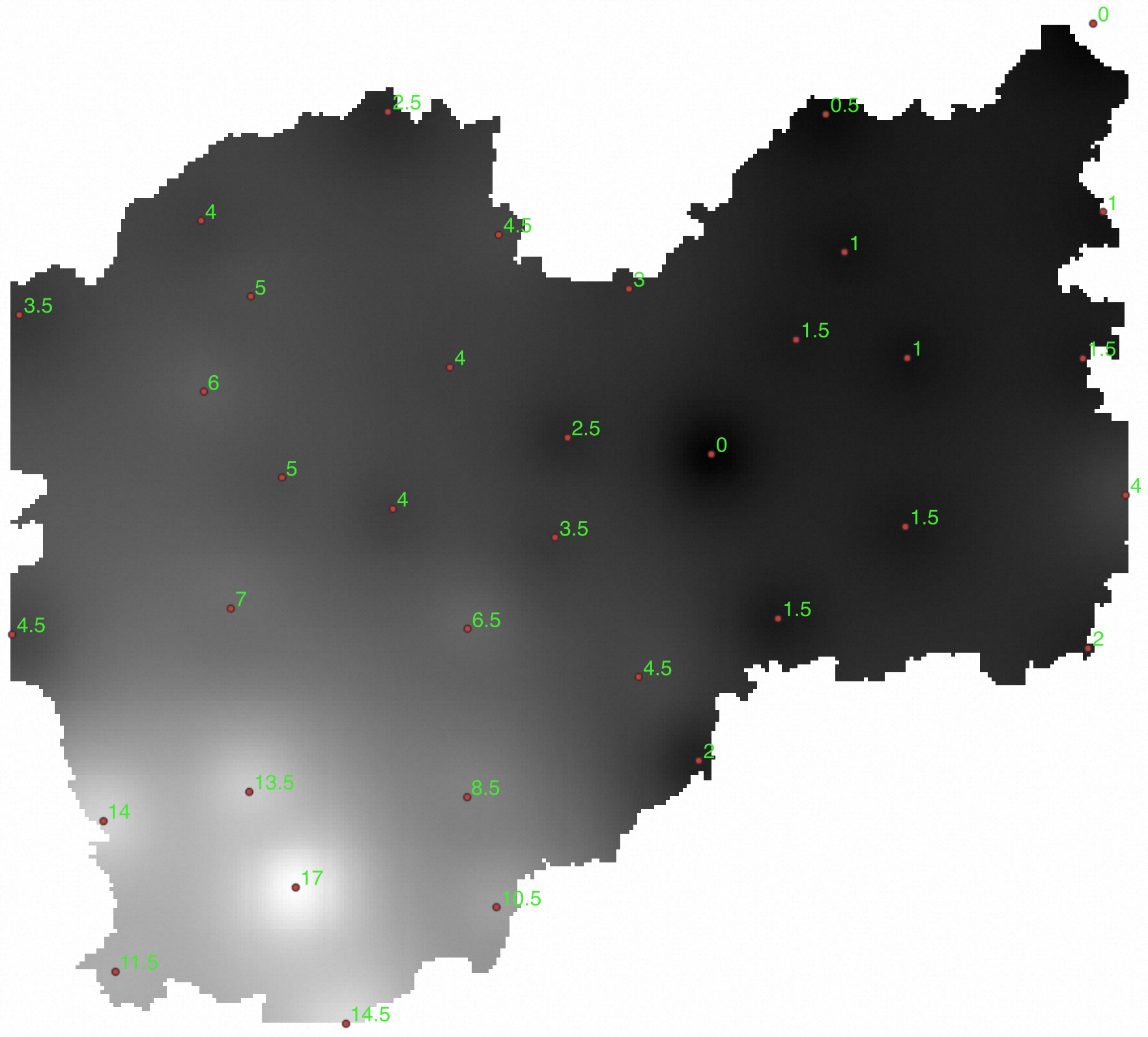
Generate contours and surfaces
ST_Contour generates both contour lines and filled polygon surfaces from a raster.
Contour lines (
"polygonize":"false", the default): Each output feature is a line geometry at the specified contour value.Filled surfaces (
"polygonize":"true"): Each output feature is a non-overlapping polygon that covers the area between two adjacent contour values. For example, with an interval of 1.0, one polygon covers the region where values fall between 2.0 and 3.0, another covers 3.0 to 4.0, and so on.
Generate contour lines
The following statement generates contour lines at an interval of 1.0 unit, clips them to the administrative polygon, and stores the result in rs_contours:
CREATE TABLE rs_contours AS
SELECT id, max_value, min_value, ST_Intersection(a.geom,p.geom) FROM
(SELECT (ST_Contour(rast,1,'{"interval":"1.0"}')).*
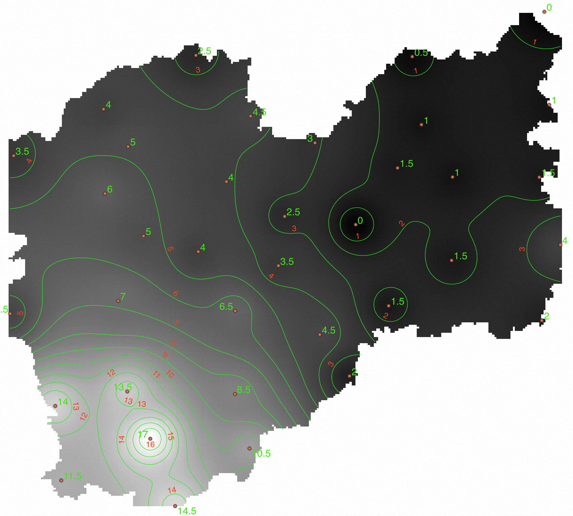
FROM raster_table WHERE id=1) a, polygon_table AS p;Import rs_contours into QGIS for an overlay display. In the image below, green numbers are measured values at observation sites and red numbers are contour values:
Generate filled surfaces
Add "polygonize":"true" to produce filled polygon surfaces instead of lines. Each output polygon covers the region between two adjacent contour values:
CREATE TABLE rs_contours_polygon AS
SELECT id, max_value, min_value, ST_Intersection(a.geom,p.geom) FROM
(SELECT (ST_Contour(rast,1,'{"interval":"1.0","polygonize":"true"}')).*
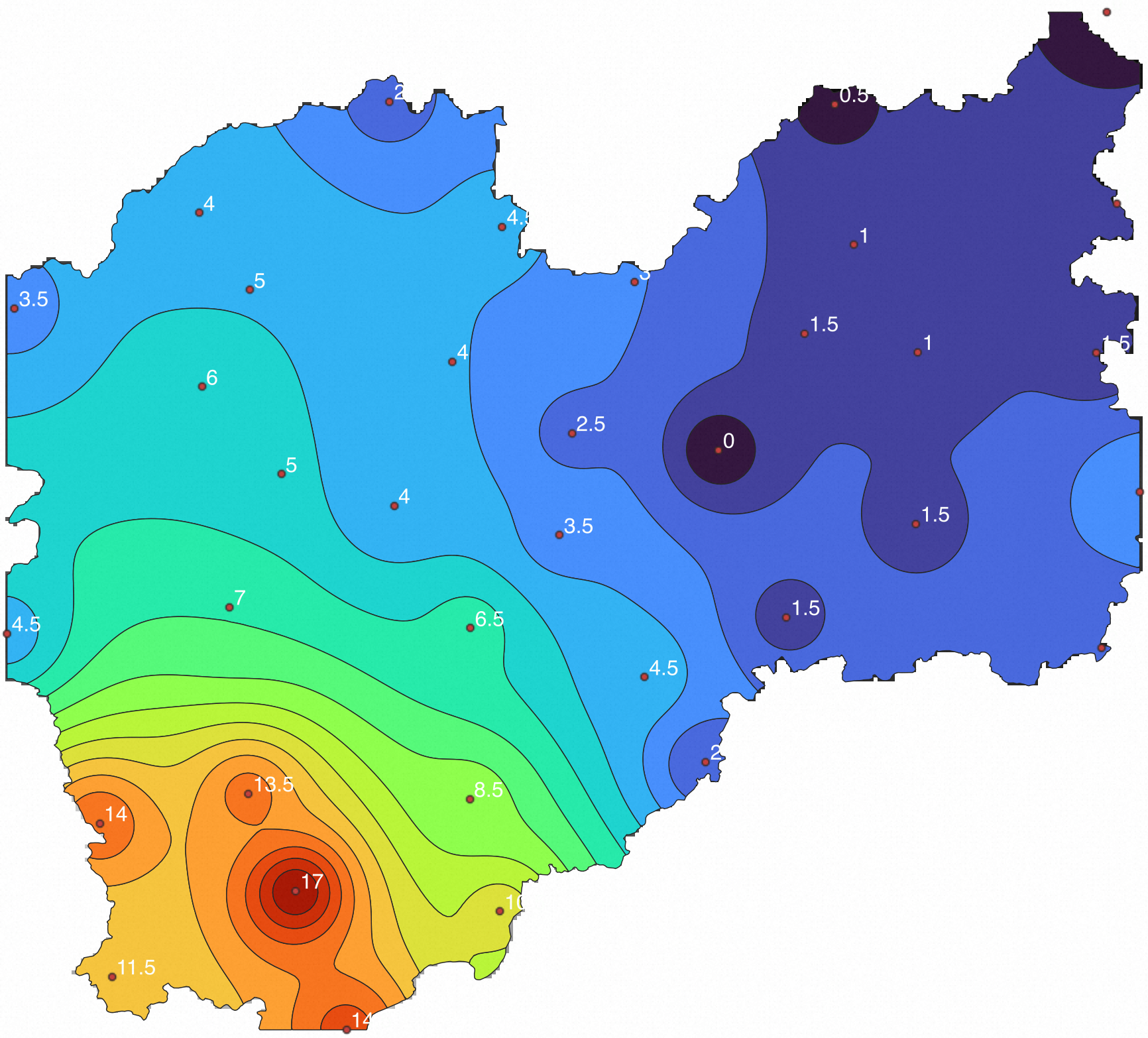
FROM raster_table WHERE id=1) a, polygon_table AS p;The following image shows the filled surfaces colored and overlaid in QGIS:
Calculate areal precipitation
Areal precipitation refers to the ratio of the total amount of precipitation within a specific area to the area of that region, usually expressed in millimeters per square meter (mm/m²). The calculation works as follows:
For each raster pixel that falls within the polygon, compute its geographic area (in m²).
Multiply the pixel's precipitation value by its area.
Sum those products across all pixels, then divide by the total pixel area.
Step 1: Review zonal statistics
Before pixel-level traversal, use ST_Statistics to get an overview of precipitation distribution within the target polygon. This function accepts a polygon geometry and a value range string, and returns per-interval statistics.
The (0,5,10,15,20] range string defines four half-open intervals: (0–5], (5–10], (10–15], and (15–20].
SELECT (ST_Statistics(rast, ST_GeomFromText('POLYGON((119.0969 28.0519, 118.9058 27.8942, 119.0502 27.5649, 119.3347 27.6292, 119.4262 27.8775, 119.4927 28.1823, 119.3812 28.1186, 119.0969 28.0519))'),
  0, '(0,5,10,15,20]',false)).*
FROM raster_table
WHERE id=1;
Expected output:
name     | band |        min         |        max         |        mean        |        sum         | count |        std         |       median       |        mode
---------+------+--------------------+--------------------+--------------------+--------------------+-------+--------------------+--------------------+--------------------
 full    |    0 | 2.5009584426879883 | 16.841625213623047 |  6.618387373747887 | 243748.58858776093 | 36829 | 2.6857099819905033 |  6.045845985412598 |  3.892089605331421
 (0-5]   |    0 | 2.5009584426879883 |  4.999907970428467 |  4.144016098134749 | 50963.109974861145 | 12298 | 0.5534420165252167 |  4.231814861297607 |  3.892089605331421
 (5-10]  |    0 |  5.000039577484131 |  9.999935150146484 |  6.852788502446667 |  136110.0852355957 | 19862 | 1.2932534814382863 |  6.623260498046875 |  5.028009414672852
 (10-15] |    0 |  10.00007438659668 | 14.993864059448242 | 11.947531793007881 |  52999.25103378296 |  4436 | 1.2279701295194279 | 11.900737762451172 | 12.430845260620117
 (15-20] |    0 |  15.00446891784668 | 16.841625213623047 | 15.777434950734413 |  3676.142343521118 |   233 | 0.5092360295014834 |   15.7352294921875 |  15.00446891784668
(5 rows)
From this output: the maximum precipitation in the area is 16.84 mm, the minimum is 2.5 mm, and there are 4,436 pixels with precipitation amounts greater than 10 mm but less than or equal to 15 mm.
Step 2: Clip the raster to the target polygon
Clip the raster to the target polygon and store the result as id=3:
INSERT INTO raster_table
SELECT 3, ST_ClipToRast(rast, ST_GeomFromText('POLYGON((119.0969 28.0519, 118.9058 27.8942, 119.0502 27.5649, 119.3347 27.6292, 119.4262 27.8775, 119.4927 28.1823, 119.3812 28.1186, 119.0969 28.0519))'),
  0, '', NULL, '', '{"chunktable":"rbt"}')
FROM raster_table WHERE id=1;
Get the pixel dimensions of the clipped raster to determine the traversal bounds:
SELECT ST_Width(rast), ST_Height(rast) FROM raster_table WHERE id=3;Expected output:
st_width  | st_height
----------+-----------
      185 |       217
Step 3: Get the area and precipitation value for each pixel
Create a table to store per-pixel data:
CREATE TABLE pixel_pre
(
   row integer,
   col integer,
   geom geometry, -- pixel area
   pre  double precision -- pixel value
);

UPDATE raster_table SET rast=ST_SetSrid(rast, 4326);

-- Traverse each pixel of the clipped raster to get its covered area and precipitation value
DO
$do$
BEGIN
   FOR i IN 0..184 LOOP
      FOR j IN 0..216 LOOP
            INSERT INTO pixel_pre
            SELECT i,j, ST_PixelAsPolygon(rast,j,i),ST_Value(rast,0,i,j) as value FROM raster_table where id=3;
      END LOOP;
   END LOOP;
END
$do$;
This pixel-level loop is necessary because it computes the precise geographic area of each pixel polygon individually. ST_Statistics returns aggregate statistics but does not provide per-pixel area weights needed for the final calculation.Verify the pixel data:
SELECT ROW,col,ST_AsText(geom),pre FROM pixel_pre LIMIT 10;Expected output (each row shows the row/column index, the polygon geometry of the pixel, and its precipitation value):
row  | col |                                                                                    st_astext                                                                                     |        pre
-----+-----+----------------------------------------------------------------------------------------------------------------------------------------------------------------------------------+--------------------
 107 |  33 | POLYGON((119.244752593338 28.0907410103828,119.244752593338 28.0878755431622,119.2479422912 28.0878755431622,119.2479422912 28.0907410103828,119.244752593338 28.0907410103828)) |   5.66606330871582
 107 |  34 | POLYGON((119.244752593338 28.0878755431622,119.244752593338 28.0850100759417,119.2479422912 28.0850100759417,119.2479422912 28.0878755431622,119.244752593338 28.0878755431622)) |  5.698885917663574
 107 |  35 | POLYGON((119.244752593338 28.0850100759417,119.244752593338 28.0821446087211,119.2479422912 28.0821446087211,119.2479422912 28.0850100759417,119.244752593338 28.0850100759417)) | 5.7316670417785645
 107 |  36 | POLYGON((119.244752593338 28.0821446087211,119.244752593338 28.0792791415006,119.2479422912 28.0792791415006,119.2479422912 28.0821446087211,119.244752593338 28.0821446087211)) |  5.764394283294678
 107 |  37 | POLYGON((119.244752593338 28.0792791415006,119.244752593338 28.0764136742801,119.2479422912 28.0764136742801,119.2479422912 28.0792791415006,119.244752593338 28.0792791415006)) |  5.797055244445801
 107 |  38 | POLYGON((119.244752593338 28.0764136742801,119.244752593338 28.0735482070595,119.2479422912 28.0735482070595,119.2479422912 28.0764136742801,119.244752593338 28.0764136742801)) |  5.829642295837402
 107 |  39 | POLYGON((119.244752593338 28.0735482070595,119.244752593338 28.070682739839,119.2479422912 28.070682739839,119.2479422912 28.0735482070595,119.244752593338 28.0735482070595))   |  5.862148761749268
 107 |  40 | POLYGON((119.244752593338 28.070682739839,119.244752593338 28.0678172726184,119.2479422912 28.0678172726184,119.2479422912 28.070682739839,119.244752593338 28.070682739839))    |  5.894571304321289
 107 |  41 | POLYGON((119.244752593338 28.0678172726184,119.244752593338 28.0649518053979,119.2479422912 28.0649518053979,119.2479422912 28.0678172726184,119.244752593338 28.0678172726184)) |   5.92690896987915
 107 |  42 | POLYGON((119.244752593338 28.0649518053979,119.244752593338 28.0620863381773,119.2479422912 28.0620863381773,119.2479422912 28.0649518053979,119.244752593338 28.0649518053979)) |  5.959161758422852
(10 rows)
Step 4: Calculate weighted areal precipitation
Raster pixels in EPSG:4326 (geographic coordinates) have areas that vary with latitude, so convert each pixel polygon to EPSG:3857 (metric projection) before computing its area in square meters. Then compute the area-weighted average:
SELECT sum(ST_Area(ST_Transform(geom,3857)) * pre) / sum(ST_Area(ST_Transform(geom,3857))) as "precipitation(mm/m^2)"
FROM pixel_pre WHERE pre>0;
Expected output:
precipitation(mm/m^2)
-----------------------
     9.434021577002174
(1 row)
The areal precipitation for this polygon is approximately 9.43 mm/m².
Conclusion
GanosBase Raster provides a complete in-database pipeline for raster data — import, storage, spatial analysis, and visualization. It meets the requirements of remote sensing image management, DEM data analysis, and grid data analysis, and offers advanced capabilities like GPU computation to support various applications. This tutorial demonstrated an end-to-end areal precipitation workflow covering FDW-based data import, IDW interpolation, boundary clipping, contour and surface generation, zonal statistics, and pixel-level area-weighted calculation. The use of GanosBase raster engine in areal precipitation calculation has effectively supported the operation of the meteorological precipitation consultation system of the Ministry of Water Resources and has improved the analysis and calculation efficiency of the system by more than 10 times. With comprehensive capabilities across water resources, natural resources, meteorology, environmental protection, and emergency response, GanosBase raster engine provides robust spatio-temporal foundational support for aerospace big data management applications to multiple customers.
What's next
ST_InterpolateRaster — full parameter reference for spatial interpolation
ST_Contour — contour and surface generation options
ST_Statistics — zonal statistics function reference
ST_ClipToRast — raster clipping function reference
FDW quick start — importing external data with ganos_fdw