Semi-join overview and usage - PolarDB - Alibaba Cloud Documentation Center

You can use a semi-join to optimize subqueries, reduce query executions, and improve performance. This topic covers the fundamentals of semi-joins and their usage.

Prerequisites

Your PolarDB cluster must be a PolarDB for MySQL 8.0 cluster running one of the following revision versions:

8.0.1.0.5 or later.
8.0.2.2.7 or later.

To check your cluster version, see Query the engine version.

Background

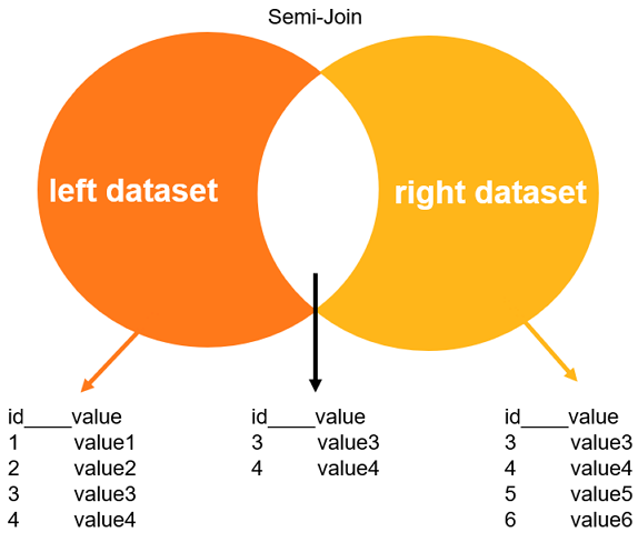
MySQL 5.6.5 introduced the semi-join optimization. When a semi-join finds a match for an outer table row in the inner table, it returns the row from the outer table. Even if multiple matches exist in the inner table, the outer table row is returned only once. This is more efficient than a standard subquery, which may re-execute the subquery for each qualifying row in the outer table. A semi-join improves performance by converting the subquery into a join. The optimizer can then process the inner and outer tables together, greatly reducing query execution time.

Strategies

A semi-join is implemented using one of the following strategies:

DuplicateWeedout strategy

This strategy creates a temporary table with unique IDs based on the row id to eliminate duplicates.

explain select * from t1 where a in (select a from t11);
id  select_type  table  partitions  type  possible_keys  key  key_len  ref  rows  filtered  Extra
1 SIMPLE  t11  NULL  ALL  NULL  NULL  NULL  0  0.00  Start temporary
1 SIMPLE  t1  NULL  ALL  NULL  NULL  NULL  3  33.33  Using where; End temporary; Using join buffer (hash join)
Warnings:
Note  1003  /* select#1 */ select `test`.`t1`.`a` AS `a`,`test`.`t1`.`b` AS `b`  from `test`.`t1` semi join (`test`.`t11`) where (`test`.`t1`.`a` = `test`.`t11`.`a`)

Materialization strategy

This strategy materializes the nested tables of a subquery into a temporary table. The optimizer then eliminates duplicates by looking up or scanning this materialized table when joining with the outer table.

explain select * from t1 where a in (select a from t11);
id  select_type table partitions  type  possible_keys key key_len ref rows  filtered  Extra
1 SIMPLE  <subquery2> NULL  ALL NULL  NULL  NULL  NULL 0.00  NULL
1 SIMPLE  t1  NULL  ALL NULL  NULL  NULL  NULL  3 33.33 Using where; Using join buffer (hash join)
2 MATERIALIZED  t11 NULL  ALL NULL  NULL  NULL  NULL  0 0.00  NULL
Warnings:
Note  1003 /* select#1 */ select `test`.`t1`.`a` AS `a`,`test`.`t1`.`b` AS `b` from `test`.`t1` semi join (`test`.`t11`) where (`test`.`t1`.`a` = `<subquery2>`.`a`)

Firstmatch strategy

This strategy performs a sequential scan. After finding the first matching row, it immediately proceeds to the next row of the outer table, thereby eliminating duplicates.

When you run an EXPLAIN statement to view the query plan, FirstMatch(t1) in the Extra column indicates that the optimizer has chosen the FirstMatch semi-join strategy.

explain select * from t1 where a in (select a from t11);
id  select_type  table  partitions  type  possible_keys  key  key_len  ref  rows  filtered  Extra
1 SIMPLE  t1  NULL  ALL NULL  NULL  NULL  NULL  3 100.00  NULL
1 SIMPLE  t11  NULL  ALL NULL  NULL  NULL  NULL  0 0.00  Using where; FirstMatch(t1); Using join buffer (hash join)
Warnings:
Note  1003  /* select#1 */ select `test`.`t1`.`a` AS `a`,`test`.`t1`.`b` AS `b` from `test`.`t1` semi join (`test`.`t11`) where (`test`.`t11`.`a` = `test`.`t1`.`a`)

LooseScan strategy

This strategy groups the inner table based on an index. It then joins each group with the outer table to find matching join conditions. If a match is found, the query returns the row from the outer table, and the scan proceeds to the next group in the inner table. This method avoids processing duplicate inner table rows.

In the EXPLAIN output, Using index; LooseScan in the Extra column for table t3 indicates that the subquery was optimized into a semi-join using the LooseScan strategy.
```
explain select count(a) from t2 where a in ( SELECT  a FROM t3);
id  select_type table partitions  type  possible_keys key key_len ref rows   filtered  Extra
1 SIMPLE  t3  NULL  index  a a 5 NULL  30000 3.33  Using where; Using index; LooseScan
1 SIMPLE  t2  NULL  ref  a a 5 test.t3.a 1 100.00  Using index
Warnings:
Note  1003 /* select#1 */ select count(`test`.`t2`.`a`) AS `count(a)` from `test`.`t2` semi join (`test`.`t3`) where (`test`.`t2`.`a` = `test`.`t3`.`a`)
```

Syntax

An IN or EXISTS subquery typically triggers a semi-join.

SELECT * FROM Employee WHERE DeptName IN (   SELECT DeptName   FROM Dept )

EXISTS

SELECT * FROM Employee WHERE EXISTS (   SELECT 1   FROM Dept   WHERE Employee.DeptName = Dept.DeptName )

Parallel semi-join performance

For queries that use a semi-join strategy, PolarDB provides parallel acceleration for all semi-join strategies. It splits a semi-join task into a set of subtasks that run concurrently using a multi-threading model. This enhances the deduplication capability and significantly improves query performance. Starting from PolarDB 8.0.2.2.7, multi-phase parallel query is supported for the Materialization strategy, further boosting semi-join performance. The following Q20 example demonstrates this.

SELECT
   s_name,
   s_address 
FROM
   supplier,
   nation 
WHERE
   s_suppkey IN 
   (
      SELECT
         ps_suppkey 
      FROM
         partsupp 
      WHERE
         ps_partkey IN 
         (
            SELECT
               p_partkey 
            FROM
               part 
            WHERE
               p_name LIKE '[COLOR]%' 
         )
         AND ps_availqty > ( 
         SELECT
            0.5 * SUM(l_quantity) 
         FROM
            lineitem 
         WHERE
            l_partkey = ps_partkey 
            AND l_suppkey = ps_suppkey 
            AND l_shipdate >= date('[DATE]') 
            AND l_shipdate < date('[DATE]') + interval '1' year ) 
   )
   AND s_nationkey = n_nationkey 
   AND n_name = '[NATION]' 
ORDER BY
   s_name;

In this example, both the subquery and the outer query execute in parallel with a degree of parallelism (DOP) of 32. The subquery first generates a materialized table in parallel. The outer query then also runs in parallel. This approach fully utilizes CPU processing power to maximize query parallelism. The following shows the multi-phase parallel processing capability in a hot data scenario with a TPC-H dataset at a 100 GB scale.

Note

The TPC-H implementation in this topic is based on TPC-H benchmarking. These test results cannot be compared with published TPC-H benchmark results because the tests do not meet all TPC-H requirements.

The parallel query plan is as follows:

 -> Sort: <temporary>.s_name  (cost=5014616.15 rows=100942)
    -> Stream results
        -> Nested loop inner join  (cost=127689.96 rows=100942)
            -> Gather (slice: 2; workers: 64; nodes: 2)  (cost=6187.68 rows=100928)
                -> Nested loop inner join  (cost=1052.43 rows=1577)
                    -> Filter: (nation.N_NAME = 'KENYA')  (cost=2.29 rows=3)
                        -> Table scan on nation  (cost=2.29 rows=25)
                    -> Parallel index lookup on supplier using SUPPLIER_FK1 (S_NATIONKEY=nation.N_NATIONKEY), with index condition: (supplier.S_SUPPKEY is not null), with parallel partitions: 863  (cost=381.79 rows=631)
            -> Single-row index lookup on <subquery2> using <auto_distinct_key> (ps_suppkey=supplier.S_SUPPKEY)
                -> Materialize with deduplication
                    -> Gather (slice: 1; workers: 64; nodes: 2)  (cost=487376.70 rows=8142336)
                        -> Nested loop inner join  (cost=73888.70 rows=127224)
                            -> Filter: (part.P_NAME like 'lime%')  (cost=31271.54 rows=33159)
                                -> Parallel table scan on part, with parallel partitions: 6244  (cost=31271.54 rows=298459)
                            -> Filter: (partsupp.PS_AVAILQTY > (select #4))  (cost=0.94 rows=4)
                                -> Index lookup on partsupp using PRIMARY (PS_PARTKEY=part.P_PARTKEY)  (cost=0.94 rows=4)
                                -> Select #4 (subquery in condition; dependent)
                                    -> Aggregate: sum(lineitem.L_QUANTITY)
                                        -> Filter: ((lineitem.L_SHIPDATE >= DATE'1994-01-01') and (lineitem.L_SHIPDATE < <cache>((DATE'1994-01-01' + interval '1' year))))  (cost=4.05 rows=1)
                                            -> Index lookup on lineitem using LINEITEM_FK2 (L_PARTKEY=partsupp.PS_PARTKEY, L_SUPPKEY=partsupp.PS_SUPPKEY)  (cost=4.05 rows=7)

In a standard TPC-H hot data scenario at 100 GB scale, the serial execution time is:

| Supplier#000999085 | egFwcBv5TkH                                  |
| Supplier#000999105 | 1CKYsKKIxqM                                  |
| Supplier#000999253 | q0nlouqFchhsbmkPq                            |
| Supplier#000999314 | 1MLMPBBnYSnMl1lRRjXiu2B2sxahjItRt0v          |
| Supplier#000999319 | hkc5LIrtAz9clk2Edz8ENngn4PdhcSD02YRxN        |
| Supplier#000999347 | L,CPr2clOoPg91gYxqCsie7DNf                   |
| Supplier#000999357 | tQW7OYPfNDzfqqzHQCx                          |
| Supplier#000999362 | X7 Rxrst808LeHI1sYlVIW5Usqu                  |
| Supplier#000999394 | TZn2ZOsZCxMmW09                              |
| Supplier#000999486 | SMiqFfRyUuXldJp                              |
| Supplier#000999684 | SwmVOJNeJwTdDJcE0                            |
| Supplier#000999814 | Tlh9Z1u5EPk1drhEbiTZpRHJJwTX3FwJoE           |
| Supplier#000999841 | 9e5iYCk2pntVLLKnP5YJ3xT2IY0I7gENyfqy        |
| Supplier#000999850 | XEzRaermdYPO5XX                              |
| Supplier#000999902 | D4XvfAYuocmiUFM1N,EScgAHQcF                  |
| Supplier#000999936 | GkUI05zvDkNpMPlE,AplBgF8PxfEhe               |
| Supplier#000999949 | bRcyGJoAryorYRUKGtYfNt4ZlgvC6vZ              |
| Supplier#000999956 | 5r fovH1Bwu087yF5L7YHitAZWtmK                |
| Supplier#000999969 | 0xHYbgscQREncmbZziaM3dxg51jA,PKhyrAQ         |
+--------------------+----------------------------------------------+
17978 rows in set (43.52 sec)

With multi-node parallel execution enabled, the execution time is:

| Supplier#000999085 | egFwcBv5TkH                                |
| Supplier#000999105 | 1CKYsKKIxqM                                |
| Supplier#000999253 | q0nlouqFchhsbmkPq                          |
| Supplier#000999314 | 1MLMPBBnYSnMl1lRRjXiu2B2sxahjItRt0v        |
| Supplier#000999319 | hkc5LIrtAz9clk2Edz8ENngn4PdhcSD02YRxN      |
| Supplier#000999347 | L,CPr2cl0oPg91gYxqCsie7DNf                 |
| Supplier#000999357 | tQW7OYPfNDzfqqzHQCx                        |
| Supplier#000999362 | X7 Rxrst808LeHI1sYlVIW5Usqu                |
| Supplier#000999394 | TZn2ZOsZCxMmW09                            |
| Supplier#000999486 | SMiqFfRyUuXldJp                            |
| Supplier#000999684 | SwmVOJNeJwTdDJcE0                          |
| Supplier#000999814 | Tlh9Z1u5EPk1drhEbiTZpRHJJwTX3FwJoE         |
| Supplier#000999841 | 9e5iYCk2pntVLLKnP5YJ3xT2IY0I7gENyfqy      |
| Supplier#000999850 | XEzRaermdYPO5XX                            |
| Supplier#000999902 | D4XvfAYuocmiUFM1N,EScgAHQcF                |
| Supplier#000999936 | GkUI0SzvDkNpMPlE,AplBgF8PxfEhe             |
| Supplier#000999949 | bRcyGJoAryorYRUKGtYfNt4ZlgvC6vZ            |
| Supplier#000999956 | 5r fovH1Bwu087yF5L7YHitAZWtmK              |
| Supplier#000999969 | 0xHYbgscQREncmbZziaM3dxg51jA,PKhyrAQ       |
17978 rows in set (2.29 sec)

The execution time decreased from 43.52 seconds to 2.29 seconds, a 19-fold performance improvement.