PolarDB:OpenSearch protocol: Performance on the hundred-million-scale MSMARCO dataset

Cluster specifications and versions

• Master node: 2-core 8 GB.

• Read-only node: 2-core 8 GB.

• Search nodes: 32-core 256 GB × 3.

• Client latency: 0.097 ms.

• PolarDB vector index version: 2.19.3.

Dataset

Create an HNSW index and write data

1. Create an index: Use the following configuration to create an index for a hundred-million-scale dataset. This configuration balances build speed, memory usage, and query performance.

   1. Define the index schema and key parameters.

      • number_of_shards: Set to 18 to distribute data and computing workloads evenly across three search nodes (96 physical cores in total).

      • ef_construction and m: These are key parameters for building an HNSW index. In this test, 128 and 8 are used to balance build speed and index quality.

      • refresh_interval and durability: These are specific optimizations to maximize test performance and are not recommended for direct use in a production environment. For more information, see Going live.

   2. Run the following command to create the index.

      curl -X PUT "http://<endpoint>:<port>/msmarco" -H 'Content-Type: application/json' -d'
      {
        "mappings": {
          "properties": {
            "docid": { "type": "keyword" },
            "domain": { "type": "keyword" },
            "emb": {
              "type": "knn_vector",
              "dimension": 1024,
              "method": {
                "engine": "faiss",
                "space_type": "l2",
                "name": "hnsw",
                "parameters": {
                  "ef_construction": 128,
                  "m": 8
                }
              }
            },
            "url": { "type": "text" }
          }
        },
        "settings": {
          "index": {
            "replication": { "type": "DOCUMENT" },
            "refresh_interval": "0s",
            "number_of_shards": "18",
            "translog": {
              "flush_threshold_size": "1gb",
              "sync_interval": "30s",
              "durability": "async"
            },
            "knn.algo_param": { "ef_search": "64" },
            "provided_name": "msmarco",
            "knn": "true",
            "number_of_replicas": "0"
          }
        }
      }
      '

2. Write data: Write the MSMARCO V2.1 dataset to the HNSW index.

Run a query performance test

The query throughput (QPS), latency, and recall rate were tested using different combinations of concurrency and the ef_search parameter.

• concurrency: Simulates from 1 to 128 concurrent queries.

• ef_search: The breadth of neighbor nodes searched in the HNSW graph during a query. A larger value theoretically results in a higher recall rate but also increases computational overhead, which decreases QPS and increases latency.

# Example command. Replace it with your actual script.
python benchmark.py --concurrency 1/2/4/8/16/32/64/128 --ef-search 32/64/128/256 --max-duration 60

Analysis of performance results

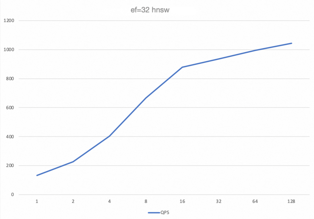
• Concurrency scalability: The QPS curve shows that as concurrency increases from 1 to 64, system throughput (QPS) grows almost linearly. This indicates that the PolarDB vector engine has good horizontal scalability. Beyond a concurrency of 64, QPS growth slows and peaks at a concurrency of 128. At this point, system resources, most likely the CPU, are nearly saturated and have become the performance bottleneck.

• Relationship between latency and concurrency: The average (Avg) and P99 latencies increase significantly as concurrency grows. This behavior is expected as the system load increases. In scenarios that require high QPS, ensure that the P99 latency meets your business requirements.

• Recall rate performance: Under all test conditions, the recall rate remains stable above 95.8%. This indicates that the HNSW index has high search accuracy with the current parameters.

Production recommendations for key parameters

The following parameters were set to achieve maximum test performance. Evaluate them carefully before using them in a production environment.

• "refresh_interval": "0s"

  • Test purpose: To disable auto-refresh. This ensures that during the write test, data is written only to memory and the translog. A manual refresh is run before the query test to obtain query performance data without interference from background tasks.

  • Production recommendation: Do not set this to 0s in a production environment. Set a reasonable value based on your data visibility requirements. For example, a value of 1s means that new data is searchable approximately 1 second after it is written.

• "durability": "async"

  • Test purpose: To use asynchronous translog flushing. Data is written to memory and a success response is returned immediately. A background thread then asynchronously persists the data to disk. This improves write throughput.

  • Production recommendation: Use this with caution in scenarios that require high data reliability. In extreme situations, such as a server breakdown, the async mode can lead to the loss of the last few seconds of data that has not been persisted to disk. If you have high data reliability requirements, use the default request mode in your production environment. This mode ensures that a success response is returned only after data is written to the translog and persisted to the disk, but it reduces write performance.

Resource utilization assessment

Understanding the system's resource consumption under peak load is crucial for accurate capacity planning.

• Write-intensive scenarios: During peak writes at 8,394 docs/sec, the primary system bottlenecks are CPU (used for index construction) and disk I/O (used for translog writes).

• Query-intensive scenarios: During peak queries at a concurrency of 128 and 1,067 QPS, the system bottleneck is primarily CPU usage.