PolarDB:Implementation of the GroupJoin operator in IMCI

Background

SELECT
  key1,
  SUM(sales) as total_sales
FROM
  fact_table LEFT JOIN dimension_table ON fact_table.key1 = dimension_table.key1
GROUP BY
  fact_table.key1
ORDER BY
  total_sales
LIMIT 100;

In PolarDB IMCI, the execution plan for a query like the preceding one typically runs a HASH JOIN first and then a HASH GROUP BY on key1. Both operations build a hash table on key1 (note that fact_table.key1 = dimension_table.key1). The execution plan is as follows:

1. HASH JOIN: Builds a hash table on dimension_table.key1, probes it with fact_table.key1, and outputs the matching data.

2. HASH GROUP BY: Builds another hash table on fact_table.key1 and performs aggregation while writing to the hash table.

From a performance perspective, these two operations can be fused into one: build a hash table on dimension_table.key1 while performing aggregation, then probe it with fact_table.key1 to continue the aggregation. This saves the time required to build a hash table on fact_table.key1. This fused operation, which merges the HASH JOIN and HASH GROUP BY operators, is called the GroupJoin operator.

Fusing these two operations eliminates one hash table build. It also reduces the size of intermediate results. A JOIN operation can potentially expand the result set, as one row from a table may match multiple rows in another. In the worst-case scenario, this leads to a Cartesian product: joining an N-row table with an M-row table can produce up to an N×M result set. With a standard HASH JOIN followed by a HASH GROUP BY, an N-row hash table might output N×M×S rows (where S is selectivity, 0 ≤ S ≤ 1). These rows are then aggregated into a new hash table, which wastes resources. Even in the preceding example of a LEFT OUTER JOIN between a large fact table (M rows) and a small dimension table (N rows) where key1 is a unique key, the process still outputs M rows from the HASH JOIN, which are then aggregated into a new hash table. In contrast, the GroupJoin operator completes the join and aggregation within the initial N-row hash table, reducing both intermediate results and memory consumption.

Based on these considerations, PolarDB for MySQL adds the GroupJoin operator to PolarDB IMCI.

Algorithm design

Overview

The GroupJoin implementation in IMCI fuses the HASH JOIN and HASH GROUP BY operators:

1. First, a hash table is built from the left (smaller) table. Aggregate functions that reference the left table are evaluated during this build phase. This process is equivalent to aggregating the left table (for example, HASH GROUP BY left_table).

2. Next, the hash table is probed using the right (larger) table. On a match, aggregate functions that reference the right table are evaluated on the corresponding hash table entry. Otherwise, the row is dropped or output directly, depending on the join type.

The following sections describe the IMCI GroupJoin algorithm in detail and discuss potential simplifications.

Limitations

To keep the implementation manageable, the PolarDB for MySQL implementation of GroupJoin has the following limitations compared to a fully generalized implementation:

1. The GROUP BY key must be the join key and must fully match the key from one of the tables. Cases where a subset of the join key can uniquely identify the key (that is, functional dependency) are not supported.

2. For RIGHT JOIN, GROUP BY RIGHT scenarios, the right-side keys must be unique. Otherwise, the optimizer may rewrite the query to LEFT JOIN, GROUP BY LEFT or avoid using the GroupJoin operator.

3. Any given aggregate function can only reference columns from either the left table or the right table, but not both. The GroupJoin operator does not apply if an aggregate function in the SELECT list references columns from both tables, such as SUM(t1.a + t2.a).

Algorithm

INNER JOIN/GROUP BY LEFT

This scenario is illustrated by the following SQL statement:

l_table INNER JOIN r_table
ON l_table.key1 = r_table.key1
GROUP BY l_table.key1

1. Build a hash table from the left table and evaluate aggregate functions that reference the left table during the build. For aggregate functions that reference the right table, maintain a "repeat count," which represents the number of matching probe-side rows for a given hash table entry.

2. During the join, probe the hash table with the right table. If a row from the right table does not find a match, it is dropped. If a match is found, increment the repeat count in the left table's aggregation context and evaluate aggregate functions that reference the right table.

3. After the join is complete, output aggregation results only for hash table entries that were matched. Unmatched entries are ignored.

4. When outputting aggregation results, account for the repeat count. For example, if a SUM(expr) result on the left table is 200 and its repeat count is 5, the final result is 1000.

INNER JOIN/GROUP BY RIGHT

This scenario is illustrated by the following SQL statement:

l_table INNER JOIN r_table
ON l_table.key1 = r_table.key1
GROUP BY r_table.key1

Because l_table.key1 = r_table.key1, this case is handled as an INNER JOIN/GROUP BY LEFT scenario.

LEFT OUTER JOIN/GROUP BY LEFT

This scenario is illustrated by the following SQL statement:

l_table LEFT OUTER JOIN r_table
ON l_table.key1 = r_table.key1
GROUP BY l_table.key1

1. Build a hash table from the left table, evaluating left-table aggregate functions during the build. For right-table aggregate functions, maintain a repeat count.

2. During the join, probe the hash table with the right table. If a row from the right table does not find a match, it is dropped. If a match is found, increment the repeat count in the left table's aggregation context and evaluate aggregate functions that reference the right table.

3. After the join is complete, output aggregation results for matched hash table entries. Unlike an INNER JOIN, each unmatched hash table entry also produces a result: it forms a separate group, and the inputs for the corresponding aggregate functions that reference the right table are NULL.

LEFT OUTER JOIN/GROUP BY RIGHT

This scenario is illustrated by the following SQL statement:

l_table LEFT OUTER JOIN r_table
ON l_table.key1 = r_table.key1
GROUP BY r_table.key1

1. Build a hash table from the left table, evaluating left-table aggregate functions during the build. For right-table aggregate functions, maintain a repeat count.

2. During the join, probe the hash table with the right table. If a row from the right table does not find a match, it is dropped. If a match is found, increment the repeat count in the left table's aggregation context and evaluate aggregate functions that reference the right table.

3. Unlike other scenarios, after the join is complete, output aggregation results for matched hash table entries. All unmatched hash table entries form a single group, and the inputs for the corresponding aggregate functions that reference the right table are NULL.

RIGHT OUTER JOIN/GROUP BY LEFT

This scenario is illustrated by the following SQL statement:

l_table RIGHT OUTER JOIN r_table
ON l_table.key1 = r_table.key1
GROUP BY l_table.key1

1. Build a hash table from the left table, evaluating left-table aggregate functions during the build. For right-table aggregate functions, maintain a repeat count.

2. Unlike other scenarios, during the join, probe the hash table with the right table. If a match is found, increment the repeat count in the left table's aggregation context and evaluate aggregate functions that reference the right table. If there is no match, all unmatched rows from the right table form a single group, where the results for the left table's aggregate functions are NULL.

3. Also unlike other scenarios, after the join is complete, output aggregation results for matched hash table entries directly. All unmatched hash table entries are ignored.

RIGHT OUTER JOIN/GROUP BY RIGHT

This scenario is illustrated by the following SQL statement:

l_table RIGHT OUTER JOIN r_table
ON l_table.key1 = r_table.key1
GROUP BY r_table.key1

Limitation

The key r_table.key1 must be distinct; otherwise, this join is invalid. If you cannot ensure that r_table.key1 is distinct, the optimizer must convert this join and group-by operation to a LEFT OUTER JOIN with a GROUP BY LEFT.

Procedure

1. Build a hash table from the left table, evaluating left-table aggregate functions during the build. For right-table aggregate functions, maintain a repeat count.

2. Unlike other scenarios, during the join, probe the hash table with the right table. If a match is found, directly output the aggregation results for both tables. If there is no match, also output the aggregation results, but the results for the left table's aggregates are all NULL.

3. Unlike other scenarios, the GroupJoin operation is complete immediately after the join finishes. No further processing of hash table entries is needed.

Handling runtime spilling

GroupJoin spilling is similar to the partition-based spilling used by HASH JOIN and HASH GROUP BY operators. The method is as follows:

1. The overall GroupJoin algorithm uses a partition-based approach.

2. When building the hash table from the left table, the algorithm for in-memory partitions is the same as described in the Algorithm section.

3. During the hash table build, partitions that do not fit in memory are spilled to corresponding temporary files on disk. New data for these partitions is also directly written to these files. A bloom filter is created for each spilled partition to quickly filter out right-table data that cannot possibly match during the probe phase.

4. After the hash table for the left table is built, probe it using data from the right table:

   1. During the probe, if the corresponding partition is in memory, it is processed as described in the Algorithm section. If the partition is not in memory, check the bloom filter first. If the data does not match the bloom filter, drop it or output it directly. Otherwise, spill the data to the temporary file for that partition.

   2. After all in-memory partitions are processed, process the on-disk partitions one by one. This assumes that at least one partition can fit in memory, so no further re-partitioning is needed. The processing algorithm is the same as described in the Algorithm section.

Related work

A 2011 paper, Accelerating Queries with Group-By and Join by Groupjoin (referred to as paper_1), discusses the theoretical feasibility of the GroupJoin operator in various execution plans but provides few implementation details. The paper describes constraints and applicable scenarios, such as how to handle different aggregate functions, but its presentation is abstract and difficult to read.

A 2021 paper, A Practical Approach to Groupjoin and Nested Aggregates (referred to as paper_2), describes how to efficiently implement the GroupJoin operator in an in-memory database. Key points include:

1. Use GroupJoin in subquery decoupling

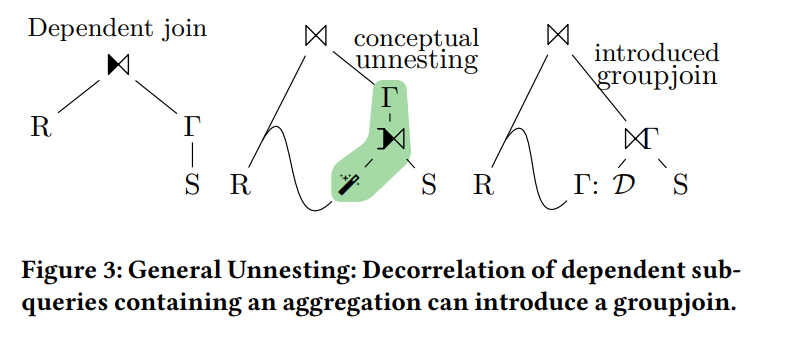
To handle correlated subqueries where a GROUP BY sits above correlated predicates, one approach is to introduce a "MagicSet" operation (a form of table distinct) and add a JOIN with a GROUP BY above it. This decouples the subquery. An execution plan of this shape is a perfect fit for the GroupJoin operator. Although IMCI uses a similar subquery decoupling method, it cannot yet generate execution plans with shared children.

2. Eager aggregation

Essentially, this means evaluating aggregate functions on the build side of the hash join during the build process, rather than storing the full payload for each hash table entry and computing the functions later. This is the same approach used in the IMCI implementation.

3. Use memoizing to handle contention during concurrent probing and aggregation

Consider an extreme case: during a hash probe, all data maps to the same entry in the hash table. This requires performing aggregation (for example, SUM(2 * col)) on this single entry, which means many threads must try to update the same "aggregation context". For a SUM() function, this involves repeatedly adding to the same sum value. Even atomic additions suffer under heavy contention, and generic aggregate functions are worse. The paper proposes a solution where each entry is assigned an owner thread using a Compare-and-Swap (CAS) instruction. Threads that fail to acquire ownership aggregate their data into private, local hash tables. These local hash tables are then merged into the global hash table at the end.

4. GroupJoin is not suitable for all scenarios

In some cases, a separate JOIN and GROUP BY perform better. For example, assume the selectivity on the hash build side is very low. After the hash probe, most rows from the build side will not be selected. This creates a dilemma:

• If you use eager aggregation during the build phase, you save memory by not storing payloads. However, with low join selectivity, most of this pre-computed aggregation work is wasted on rows that are ultimately discarded.

• If you do not perform aggregation in advance, you use more memory. However, if join selectivity is high, this extra memory could have been saved by using eager aggregation.

Therefore, if the join selectivity is low, a better approach might be to: complete the join to get a very small number of groups, and then perform a highly localized aggregation using HASH GROUP BY. The paper proposes different implementations for different scenarios. To determine which scenario a query falls into, the optimizer needs to provide selectivity and cardinality estimates, and the paper provides some estimation methods to support this.

From an implementer's perspective, this "dilemma" is not a major issue for two reasons:

• PolarDB IMCI almost always builds the hash table on the smaller side (the small table).

• Even if join selectivity is low, using eager aggregation may waste some computation on a small table, but it always saves memory. In this situation, it is a reasonable time-for-space trade-off compared to a separate HASH JOIN and HASH GROUP BY.

In the IMCI implementation, except for the RIGHT JOIN, GROUP BY RIGHT scenario described earlier, PolarDB IMCI almost always considers the GroupJoin operator to be more efficient than a separate HASH JOIN and HASH GROUP BY.

Based on the authors and experiments cited, both papers appear to come from the HyPer database team at the University of Munich. Outside of HyPer, other databases are not known to have implemented the GroupJoin operator. However, other implementations of "shared hash table" operations may exist, which is a topic for future discussion.

Use cases for GroupJoin in TPC-H

TPC-H is a common benchmark for testing the analytical query capabilities of an AP system. Many of the 22 queries in TPC-H are suitable for the GroupJoin operator. However, with the exception of TPC-H Q13, most queries require rewriting before GroupJoin can be applied.

Q13

TPC-H Q13 can use the GroupJoin operator directly:

select
    c_count,
    count(*) as custdist
from
    (
        select
            c_custkey,
            count(o_orderkey) as c_count
        from
            customer
            left outer join orders on c_custkey = o_custkey
            and o_comment not like '%pending%deposits%'
        group by
            c_custkey
    ) c_orders
group by
    c_count
order by
    custdist desc,
    c_count desc;

• In IMCI, without the GroupJoin operator, the execution plan is as follows:

  1 Project | Exprs: temp_table4.temp_table2.COUNT(orders.o_orderkey), temp_table4.COUNT(0)
  2   Sort | Exprs: temp_table4.COUNT(0) DESC,temp_table4.temp_table2.COUNT(orders.o_orderkey) DESC
  3     HashGroupby | OutputTable(4): temp_table4 | Grouping: temp_table2.COUNT(orders.o_orderkey) | Output Grouping: temp_table2.C
  4       HashGroupby | OutputTable(2): temp_table2 | Grouping: customer.c_custkey | Output Grouping: customer.c_custkey | Aggrs: C
  5         HashJoin | HashMode: DYNAMIC | JoinMode: LEFT_OUTER | JoinPred: customer.c_custkey = orders.o_custkey
  6           CTableScan | InputTable(0): customer | Pred: (TRUE PRED)
  7           CTableScan | InputTable(1): orders | Pred: ( NOT (orders.o_comment LIKE "%pending%deposits%"))

• With the GroupJoin operator, the execution plan is as follows:

  9 Project | Exprs: temp_table4.temp_table2.COUNT(orders.o_orderkey), temp_table4.COUNT(0)
  10   Sort | Exprs: temp_table4.COUNT(0) DESC,temp_table4.temp_table2.COUNT(orders.o_orderkey) DESC
  11     HashGroupby | OutputTable(4): temp_table4 | Grouping: temp_table2.COUNT(orders.o_orderkey) | Output Grouping: temp_table2.C
  12       GroupJoin | Grouping: customer.c_custkey (unique) | JoinMode: LEFT OUTER | JoinPred: customer.c_custkey = orders.o_custke
  13         CTableScan | InputTable(0): customer | Pred: (TRUE PRED)
  14         CTableScan | InputTable(1): orders | Pred: ( NOT (orders.o_comment LIKE "%pending%deposits%"))

Q3

For TPC-H Q3, enabling the GroupJoin operator requires a series of equivalence transformations:

select
    l_orderkey,
    sum(l_extendedprice * (1 - l_discount)) as revenue,
    o_orderdate,
    o_shippriority
from
    customer,
    orders,
    lineitem
where
    c_mktsegment = 'BUILDING'
    and c_custkey = o_custkey
    and l_orderkey = o_orderkey
    and o_orderdate < date '1995-03-15'
    and l_shipdate > date '1995-03-15'
group by
    l_orderkey,
    o_orderdate,
    o_shippriority
order by
    revenue desc,
    o_orderdate
limit
    10;

A feasible execution plan for Q3 in IMCI is as follows:

1  Project | Exprs: temp_table3.lineitem.l_orderkey, temp_table3.SUM(lineitem.l_extendedprice * 1.00 - lineitem.l_discount), temp_...
2    TopK | Limit = 10 | Exprs: temp_table3.SUM(lineitem.l_extendedprice * 1.00 - lineitem.l_discount) DESC,temp_table3.orders.o_orderdate
3      HashGroupby | OutputTable(3): temp_table3 | Grouping: lineitem.l_orderkey orders.o_orderdate orders.o_shippriority | Output: lineitem.l_orderkey, orders.o_orderdate, orders.o_shippriority, SUM(lineitem.l_extendedprice * 1.00 - lineitem.l_discount)
4        HashJoin | HashMode: DYNAMIC | JoinMode: INNER | JoinPred: orders.o_orderkey = lineitem.l_orderkey
5          HashJoin | HashMode: DYNAMIC | JoinMode: INNER | JoinPred: orders.o_custkey = customer.c_custkey
6            CTableScan | InputTable(0): orders | Pred: (orders.o_orderdate < 03/15/1995 00:00:00.000000)
7            CTableScan | InputTable(1): customer | Pred: (customer.c_mktsegment = "BUILDING")
8          CTableScan | InputTable(2): lineitem | Pred: (lineitem.l_shipdate > 03/15/1995 00:00:00.000000)

Because the grouping keys are l_orderkey, o_orderdate, and o_shippriority, which do not match any single join key, GroupJoin does not apply directly. However, the following can be derived through equivalence reasoning:

1. The join predicate between the lineitem and orders tables is l_orderkey = o_orderkey, and it is an INNER JOIN. Therefore, l_orderkey = o_orderkey holds for the entire result set.

2. Because l_orderkey = o_orderkey, GROUP BY l_orderkey, o_orderdate, o_shippriority is equivalent to GROUP BY o_orderkey, o_orderdate, o_shippriority.

3. Because o_orderkey is the PRIMARY KEY of the orders table, each o_orderkey uniquely determineso_orderdate and o_shippriority (that is, o_orderdate and o_shippriority functionally depend on o_orderkey).

4. Because o_orderkey uniquely determines o_orderdate and o_shippriority, GROUP BY o_orderkey, o_orderdate, o_shippriority is equivalent to GROUP BY o_orderkey.

With these deductions, the GROUP BY clause of Q3 can be rewritten to GROUP BY o_orderkey, which makes GroupJoin applicable:

Project | Exprs: temp_table3.lineitem.l_orderkey, temp_table3.SUM(lineitem.l_extendedprice * 1.00 - lineitem.l_discount), temp_
TopK | Limit = 10 | Exprs: temp_table3.SUM(lineitem.l_extendedprice * 1.00 - lineitem.l_discount) DESC,temp_table3.ANY_VALUE(orders.o_orderdate)
  GroupJoin | Grouping: lineitem.l_orderkey | JoinMode: INNER | JoinPred: orders.o_orderkey = lineitem.l_orderkey
    HashJoin | HashMode: DYNAMIC | JoinMode: INNER | JoinPred: orders.o_custkey = customer.c_custkey
      CTableScan | InputTable(0): orders | Pred: (orders.o_orderdate < 03/15/1995 00:00:00.000000)
      CTableScan | InputTable(1): customer | Pred: (customer.c_mktsegment = "BUILDING")
    CTableScan | InputTable(2): lineitem | Pred: (lineitem.l_shipdate > 03/15/1995 00:00:00.000000)

This kind of "functional dependency" deduction requires advanced optimizer support. The MySQL optimizer currently implements partial functional dependency inference but cannot derive the GROUP BY o_orderkey rewrite shown above. Experiments show that SQL Server can perform this transformation. Although the theory is well-established, IMCI has not yet fully implemented it. In TPC-H, queries Q3, Q4, Q10, Q13, Q18, Q20, and Q21 share this pattern. Applying these equivalence rewrites would shorten the GROUP BY keys and accelerate aggregation.

Q10

TPC-H Q10 also cannot directly use the GroupJoin operator:

select
    c_custkey,
    c_name,
    sum(l_extendedprice * (1 - l_discount)) as revenue,
    c_acctbal,
    n_name,
    c_address,
    c_phone,
    c_comment
from
    customer,
    orders,
    lineitem,
    nation
where
    c_custkey = o_custkey
    and l_orderkey = o_orderkey
    and o_orderdate >= date '1993-10-01'
    and o_orderdate < date '1993-10-01' + interval '3' month
    and l_returnflag = 'R'
    and c_nationkey = n_nationkey
group by
    c_custkey,
    c_name,
    c_acctbal,
    c_phone,
    n_name,
    c_address,
    c_comment
order by
    revenue desc
limit
    20;

To use the GroupJoin operator, two transformations are needed:

1. Rewrite the grouping keys to c_custkey (the PRIMARY KEY of the customer table), similar to the transformation for Q3.

2. Adjust the join order so that the join involving the customer table is the outermost join.

The first transformation is always beneficial, but adjusting the join order is not always a net positive.

Q17

TPC-H Q17 contains a correlated subquery:

select
    sum(l_extendedprice) / 7.0 as avg_yearly
from
    lineitem,
    part
where
    p_partkey = l_partkey
    and p_brand = 'Brand#44'
    and p_container = 'WRAP PKG'
    and l_quantity < (
        select
            0.2 * avg(l_quantity)
        from
            lineitem
        where
            l_partkey = p_partkey
    );

There are multiple ways to perform subquery decoupling. In IMCI, two different decoupling algorithms for scalar aggregates produce the following execution plans, neither of which can use the GroupJoin operator:

Project | Exprs: temp_table7.temp_table6.SUM(temp_table3.ANY_VALUE(lineitem.l_extendedprice)) / 7.0
  ComputeScalar | Exprs: temp_table6.SUM(temp_table3.ANY_VALUE(lineitem.l_extendedprice)) / 7.0
    HashGroupby | OutputTable(6): temp_table6 | Grouping: None | Output Grouping: None | Aggrs: SUM(temp_table3.ANY_VALUE(lineitem.l_extendedprice))
      FILTER | Pred: ((CAST temp_table3.ANY_VALUE(lineitem.l_quantity)/DECIMAL(15, 2) as DECIMAL(38, 12)) < 0.2 * temp_table3.AVG(lineitem.l_quantity))
        HashGroupby | OutputTable(3): temp_table3 | Grouping: temp_sequence.SEQUENCE_VALUE | Output Grouping: None | Aggrs: AVG(lineitem.l_quantity)
          HashJoin | HashMode: DYNAMIC | JoinMode: LEFT_OUTER | JoinPred: part.p_partkey = lineitem.l_partkey
            SEQUENCE | SequenceID: (55440)
              HashJoin | HashMode: DYNAMIC | JoinMode: INNER | JoinPred: lineitem.l_partkey = part.p_partkey
                CTableScan | InputTable(0): lineitem | Pred: (TRUE PRED)
                CTableScan | InputTable(1): part | Pred: ((part.p_brand = "Brand#44") AND (part.p_container = "WRAP PKG"))
            CTableScan | InputTable(2): lineitem | Pred: (TRUE PRED)

Project | Exprs: temp_table7.temp_table6.SUM(lineitem.l_extendedprice) / 7.0
  ComputeScalar | Exprs: temp_table6.SUM(lineitem.l_extendedprice) / 7.0
    HashGroupby | OutputTable(6): temp_table6 | Grouping: None | Output Grouping: None  | Aggrs: SUM(lineitem.l_extendedprice)
      FILTER | Pred: ((CAST lineitem.l_quantity/DECIMAL(15, 2) as DECIMAL(38, 12)) < 0.2 * temp_table3.AVG(lineitem.l_quantity))
        HashMatch | HashMode: DYNAMIC | JoinMode: LEFT_OUTER | JoinPred: part.p_partkey = temp_table3.lineitem.l_partkey
          HashJoin | HashMode: DYNAMIC | JoinMode: INNER | JoinPred: lineitem.l_partkey = part.p_partkey
            CTableScan | InputTable(0): lineitem | Pred: (TRUE PRED)
            CTableScan | InputTable(1): part | Pred: ((part.p_brand = "Brand#44") AND (part.p_container = "WRAP PKG"))
          HashGroupby | OutputTable(3): temp_table3 | Grouping: lineitem.l_partkey | Output Grouping: lineitem.l_partkey | Aggr
            CTableScan | InputTable(2): lineitem | Pred: (TRUE PRED)

However, if a MagicSet-based decoupling strategy is used, it can produce an intermediate plan shape suitable for GroupJoin before the MagicSet operator is removed:

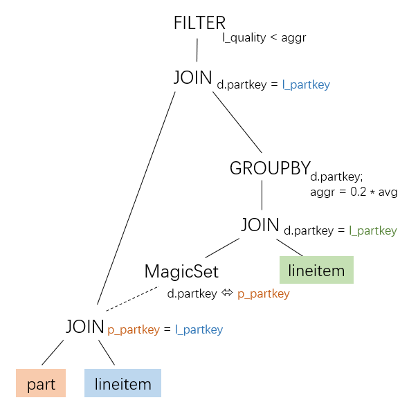
This is the process described in paper_2:

IMCI partially implements MagicSet-based decoupling but does not yet generate execution plans with shared children. Therefore, IMCI cannot apply the GroupJoin operator to TPC-H Q17.

Q18

TPC-H Q18 can also use the GroupJoin operator, but it requires equivalence transformations to produce a suitable execution plan. For simplicity, and without loss of generality, this section removes the IN subquery and the final ORDER BY clause from the original query:

select
    c_name,
    c_custkey,
    o_orderkey,
    o_orderdate,
    o_totalprice,
    sum(l_quantity)
from
    customer,
    orders,
    lineitem
where
    c_custkey = o_custkey
    and o_orderkey = l_orderkey
group by
    c_name,
    c_custkey,
    o_orderkey,
    o_orderdate,
    o_totalprice

For this query, we can apply the following equivalence reasoning:

1. Because c_custkey is the PRIMARY KEY of the customer table, c_name is functionally dependent on c_custkey. Similarly, o_orderkey is the PRIMARY KEY of the orders table, so o_orderdate and o_totalprice are functionally dependent on o_orderkey. Therefore, the GROUP BY clause is equivalent to GROUP BY c_custkey, o_orderkey.

2. The join predicate between the customer and orders tables is c_custkey = o_custkey, so we can assert that c_custkey = o_custkey in the join result set.

3. Because c_custkey = o_custkey, the GROUP BY clause can be further transformed into GROUP BY o_custkey, o_orderkey.

4. Because o_orderkey is the primary key of the orders table, it uniquely determines o_custkey. Therefore, the GROUP BY clause can be finally rewritten as GROUP BY o_orderkey.

After these transformations, the query is equivalent to the following:

select
    ANY_VALUE(c_name),
    ANY_VALUE(c_custkey),
    o_orderkey,
    ANY_VALUE(o_orderdate),
    ANY_VALUE(o_totalprice),
    sum(l_quantity)
from
    customer,
    orders,
    lineitem
where
    c_custkey = o_custkey
    and o_orderkey = l_orderkey
group by
    o_orderkey

• Execution plan without GroupJoin

  1  Project | Exprs: temp_table3.ANY_VALUE(customer.c_name), temp_table3.ANY_VALUE(customer.c_custkey), temp_table3.orders.o_orderkey, temp_table3.ANY_VALUE(orders.o_orderdate), temp_table3.ANY_VALUE(orders.o_totalprice), temp_table3.SUM(lineitem.l_quantity)
  2    HashGroupby | OutputTable(3): temp_table3 | Grouping: orders.o_orderkey | Output Grouping: orders.o_orderkey | Aggrs: ANY_VALUE(customer.c_name), ANY_VALUE(customer.c_custkey), ANY_VALUE(orders.o_orderdate), ANY_VALUE(orders.o_totalprice), SUM(lineitem.l_quantity)
  3      HashJoin | HashMode: DYNAMIC | JoinMode: INNER | JoinPred: orders.o_orderkey = lineitem.l_orderkey
  4        HashJoin | HashMode: DYNAMIC | JoinMode: INNER | JoinPred: orders.o_custkey = customer.c_custkey
  5          CTableScan | InputTable(0): orders | Pred: (TRUE PRED)
  6          CTableScan | InputTable(1): customer | Pred: (TRUE PRED)
  7        CTableScan | InputTable(2): lineitem | Pred: (TRUE PRED)

• Execution plan with GroupJoin

  1 Project | Exprs: temp_table4.ANY_VALUE(customer.c_name), temp_table4.ANY_VALUE(customer.c_custkey), temp_table4.orders.o_orderkey
  2   GroupJoin | Grouping: orders.o_orderkey | JoinMode: INNER | JoinPred: orders.o_orderkey = lineitem.l_orderkey
  3     HashJoin | HashMode: DYNAMIC | JoinMode: INNER | JoinPred: orders.o_custkey = customer.c_custkey
  4       CTableScan | InputTable(0): orders | Pred: (TRUE PRED)
  5       CTableScan | InputTable(1): customer | Pred: (TRUE PRED)
  6     CTableScan | InputTable(2): lineitem | Pred: (TRUE PRED)

These equivalence deductions are also beneficial for conventional execution plans because they shorten the GROUP BY keys.

Q20

The correlated subquery pattern in TPC-H Q20 is similar to that of Q17. Using a MagicSet-based decoupling approach produces an intermediate plan shape that is suitable for GroupJoin before the MagicSet operator is removed.

select
...
and ps_availqty > (
    select
        0.5 * sum(l_quantity) < ! --- scalar aggr --->
    from
        lineitem
    where
        l_partkey = ps_partkey         < ! --- correlated item 1 --->
        and l_suppkey = ps_suppkey     < ! --- correlated item 2 --->
        and l_shipdate >= '1993-01-01'
        and l_shipdate < date_add('1993-01-01', interval '1' year)
)

Other queries

According to paper_1 and paper_2, queries Q5, Q9, Q16, and Q21 are also suitable for the GroupJoin operator, but a suitable transformation path has not yet been found. Inspecting the execution plans of the HyPer database (https://hyper-db.de/interface.html#) shows that its optimizer also does not generate execution plans with GroupJoin for these queries.

Query performance

Many queries in the TPC-H benchmark use a JOIN + GROUP BY pattern, making them candidates for GroupJoin optimization. In paper_1, the authors report performance for queries Q3, Q5, Q9, Q10, Q13, Q16, Q17, Q20, and Q21 with and without the GroupJoin operator.

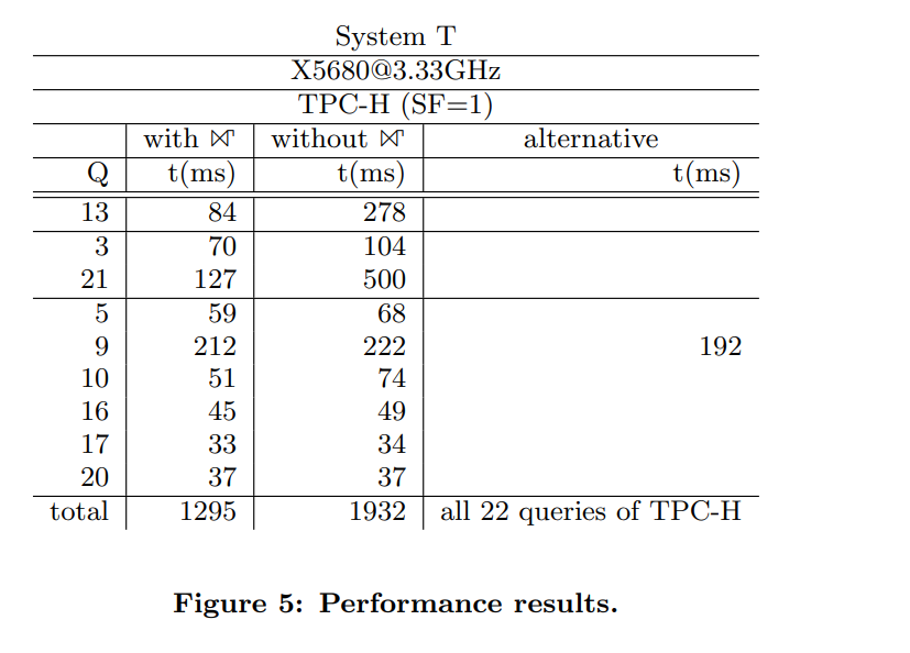
The test uses a 1 GB TPC-H dataset. The results show that the GroupJoin operator has a positive impact on TPC-H query performance, reducing the total latency from 1,932 ms to 1,295 ms.

In paper_2, the authors provide a more detailed performance breakdown for queries Q3, Q13, Q17, and Q18 across several approaches, using a 10 GB TPC-H dataset:

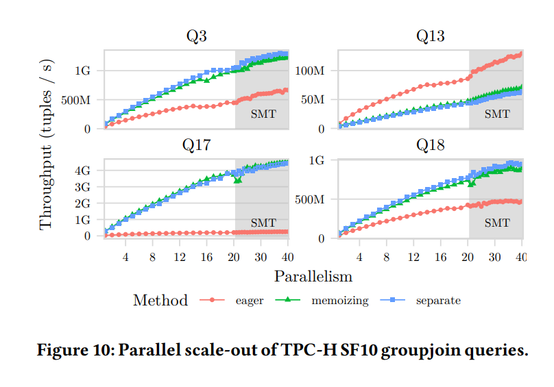
The line groups in the figure represent the following:

1. "separate" refers to performing JOIN and GROUP BY separately, that is, not using the GroupJoin operator.

2. "eager" refers to the "eager aggregation" optimization discussed earlier.

3. "memoizing" refers to the optimization for handling concurrent hash table probes and aggregations. For queries Q3, Q13, Q17, and Q18:

   1. The "memoizing" approach almost always performs similarly to the standard HASH JOIN + HASH GROUP BY method.

   2. The "eager" aggregation approach only shows an advantage for Q13.

The data shows that performance varies significantly by scenario. This supports the paper's main point that the GroupJoin execution strategy requires accurate statistics from the optimizer to choose the optimal method, rather than indiscriminately choosing a single GroupJoin algorithm or even using the GroupJoin operator at all.

However, PolarDB has a different perspective on this conclusion:

1. The paper uses tuples per second as a performance metric, but the findings in PolarDB IMCI differ. We tested the throughput (in tuples/s) of the GroupJoin operator for queries Q3, Q13, and Q18 with a concurrency of 32. The results are as follows:

   Query	Hash join + hash group by	GroupJoin
   Q3	130 MB/s	152 MB/s
   Q13	11 MB/s	33 MB/s
   Q18	315 MB/s	1 GB/s

   Note

   The GroupJoin operator cannot currently be applied to Q17 in IMCI.

   This test data is similar in magnitude to the data in the paper, but our results for each query differ slightly. Perhaps due to implementation differences, our test data from PolarDB shows that, except for the RIGHT JOIN, GROUP BY RIGHT case, the GroupJoin operator is almost always superior to HASH JOIN + HASH GROUP BY.

2. Regarding the conclusion in 3.a above, which states that the "memoizing" method almost always has performance similar to the standard HASH JOIN + HASH GROUP BY method, our observations indicate that these specific TPC-H queries have very little contention. As a result, components such as the local hash tables used by the memoizing method are rarely used at runtime. This is why the algorithm's performance on these queries is similar to that of HASH JOIN + HASH GROUP BY. Therefore, using the performance of these queries for comparison in the paper is not a meaningful comparison. PolarDB tests runtime contention by using explicit locking.

Conclusion

In practice, the GroupJoin operator avoids redundant work at runtime and can deliver significant performance gains in certain scenarios. This benefit has been verified in production workloads. From a results-oriented standpoint, the GroupJoin operator is a worthwhile implementation.

However, GroupJoin is not a general-purpose optimization. It applies only to EQUAL JOIN with GROUP BY where the grouping keys match the join keys on one side, and it imposes many constraints on aggregate functions and implementation choices. It is a specialized feature with a high implementation and maintenance cost. From a development perspective, it can be more effective to invest in optimizing the "general path" to improve SQL performance broadly, rather than building custom solutions for narrow patterns. From this viewpoint, GroupJoin is not an ideal method.

Therefore, when implementing GroupJoin, it is wise to simplify and make trade-offs. The goal should not be to build the most complete, full-featured version, but to maximize the performance and utility for the most common and impactful scenarios.