A support vector machine (SVM) is a machine learning method based on statistical learning theory. It improves a model's generalization ability through structural risk minimization, which balances the empirical risk and the confidence interval. This topic explains how to configure the Linear SVM component and includes a usage example.
Background
This Linear SVM algorithm is implemented without using a kernel function. For details on the implementation, see the "trust region method for L2-SVM" section in algorithm principles.
Limitations
The Linear SVM component supports only binary classification.
Component configuration
You can configure the parameters for the Linear SVM component using one of the following methods.
Method 1: Visual configuration
-
Input port
The Linear SVM component has one required input port that must be connected to a Read Table component.
-
Configure the component parameters on the workflow page.
Parameter type
Parameter
Required
Description
Field settings
Feature columns
Yes
The feature columns for model training. Supported data types: BIGINT and DOUBLE.
Label column
Yes
The label column for model training. Supported data types: BIGINT, DOUBLE, and STRING.
Parameter settings
Positive sample label value
No
The value that represents a positive sample. If this parameter is not specified, a value is randomly selected from the label column. Specifying this parameter is recommended for imbalanced datasets.
Positive penalty factor
No
The weight for positive samples. The default value is 1.0, and the value range is (0, +∞).
Negative penalty factor
No
The negative sample weight has a default value of 1.0 and a value range of (0, +∞).
Convergence coefficient
No
Convergence error. The default value is 0.001. The value range is (0, 1).
Execution tuning
Number of cores
No
If unspecified, the system automatically allocates resources.
Memory per core
No
The memory size for each core, in MB. If unspecified, the system automatically allocates resources.
-
Output port
Outputs a binary classification model in OfflineModel format. The output of this component connects to a Prediction component.
Method 2: PAI command
You can configure the component parameters by running a PAI command in an SQL Script component. For more information, see SQL Script.
PAI -name LinearSVM -project algo_public
    -DinputTableName="bank_data"
    -DmodelName="xlab_m_LinearSVM_6143"
    -DfeatureColNames="pdays,emp_var_rate,cons_conf_idx"
    -DlabelColName="y"
    -DpositiveLabel="0"
    -DpositiveCost="1.0"
    -DnegativeCost="1.0"
    -Depsilon="0.001";
The following table describes the parameters in the PAI command.
|
Parameter |
Required |
Default |
Description |
|
inputTableName |
Yes |
N/A |
The name of the input table. |
|
inputTablePartitions |
No |
All partitions of the input table. |
The partitions of the input table for training. The following formats are supported:
Note
To specify multiple partitions, separate them with commas (,). |
|
modelName |
Yes |
N/A |
The name of the output model. |
|
featureColNames |
Yes |
N/A |
The names of the feature columns in the input table. |
|
labelColName |
Yes |
N/A |
The name of the label column in the input table. |
|
positiveLabel |
No |
A value is randomly selected from the label column. |
The value that represents a positive sample. |
|
positiveCost |
No |
1.0 |
The weight of the positive class, also known as the positive penalty factor. The value must be in the range (0, +∞). |
|
negativeCost |
No |
1.0 |
The weight of the negative class, also known as the negative penalty factor. The value must be in the range (0, +∞). |
|
epsilon |
No |
0.001 |
The convergence coefficient. The value must be in the range (0,1). |
|
enableSparse |
No |
false |
Specifies whether the input data is in sparse format. Valid values: true and false. |
|
itemDelimiter |
No |
, (comma) |
The delimiter between KV pairs when the input table data is in sparse format. |
|
kvDelimiter |
No |
: (colon) |
The delimiter between key and value when the input table data is in sparse format. |
|
coreNum |
No |
System-allocated |
The number of compute cores. The value must be a positive integer. |
|
memSizePerCore |
No |
System-allocated |
The memory size for each core, in MB. The value must be an integer in the range [1, 65536]. |
Example
-
Import the following training data.
id
y
f0
f1
f2
f3
f4
f5
f6
f7
1
-1
-0.294118
0.487437
0.180328
-0.292929
-1
0.00149028
-0.53117
-0.0333333
2
+1
-0.882353
-0.145729
0.0819672
-0.414141
-1
-0.207153
-0.766866
-0.666667
3
-1
-0.0588235
0.839196
0.0491803
-1
-1
-0.305514
-0.492741
-0.633333
4
+1
-0.882353
-0.105528
0.0819672
-0.535354
-0.777778
-0.162444
-0.923997
-1
5
-1
-1
0.376884
-0.344262
-0.292929
-0.602837
0.28465
0.887276
-0.6
6
+1
-0.411765
0.165829
0.213115
-1
-1
-0.23696
-0.894962
-0.7
7
-1
-0.647059
-0.21608
-0.180328
-0.353535
-0.791962
-0.0760059
-0.854825
-0.833333
8
+1
0.176471
0.155779
-1
-1
-1
0.052161
-0.952178
-0.733333
9
-1
-0.764706
0.979899
0.147541
-0.0909091
0.283688
-0.0909091
-0.931682
0.0666667
10
-1
-0.0588235
0.256281
0.57377
-1
-1
-1
-0.868488
0.1
-
Import the following test data.
id
y
f0
f1
f2
f3
f4
f5
f6
f7
1
+1
-0.882353
0.0854271
0.442623
-0.616162
-1
-0.19225
-0.725021
-0.9
2
+1
-0.294118
-0.0351759
-1
-1
-1
-0.293592
-0.904355
-0.766667
3
+1
-0.882353
0.246231
0.213115
-0.272727
-1
-0.171386
-0.981213
-0.7
4
-1
-0.176471
0.507538
0.278689
-0.414141
-0.702128
0.0491804
-0.475662
0.1
5
-1
-0.529412
0.839196
-1
-1
-1
-0.153502
-0.885568
-0.5
6
+1
-0.882353
0.246231
-0.0163934
-0.353535
-1
0.0670641
-0.627669
-1
7
-1
-0.882353
0.819095
0.278689
-0.151515
-0.307329
0.19225
0.00768574
-0.966667
8
+1
-0.882353
-0.0753769
0.0163934
-0.494949
-0.903073
-0.418778
-0.654996
-0.866667
9
+1
-1
0.527638
0.344262
-0.212121
-0.356974
0.23696
-0.836038
-0.8
10
+1
-0.882353
0.115578
0.0163934
-0.737374
-0.56974
-0.28465
-0.948762
-0.933333
-
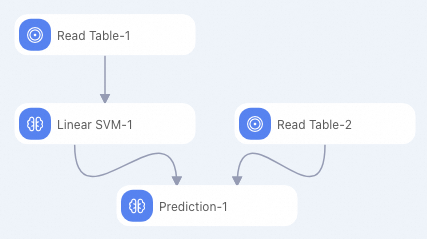
Create a pipeline as shown in the following figure. For more information, see algorithm modeling.
-
Configure the parameters for the Linear SVM component as shown in the following table. Keep the default values for all other parameters.
Parameter type
Parameter
Description
Fields Setting
Feature Columns
Select the f0, f1, f2, f3, f4, f5, f6, and f7 columns.
Label Column
Select the y column.
-
Run the pipeline and view the prediction results. After the prediction completes, the output displays the binary classification prediction results for the 10 rows of test data in five columns: id, y (actual label), prediction_result (predicted label: +1 or -1), prediction_score, and prediction_detail (score details for the +1 and -1 classes, in JSON format).