Object Storage Service:Distributed vector processing on OSS with Lance and Ray

Solution overview

This guide provides a complete implementation, using an enterprise RAG knowledge base vectorization workflow as an example. First, understand the solution's advantages and architecture, and prepare the prerequisites, such as ECS instances, OSS, and a Ray cluster. Then, configure OSS as the Lance storage backend and follow these steps to build the distributed vector data processing pipeline:

1. Prepare a unified configuration module: Centralize storage and compute parameters in a config.py file for reuse across all steps.

2. Prepare the raw dataset: Write the original text data to OSS in the Lance format.

3. Generate embeddings in a distributed manner: Use a Ray cluster to generate embeddings in parallel using an embedding model and write the results back to OSS.

4. Build a vector index and perform ANN search in a distributed manner: Construct an IVF_PQ vector index on OSS and test its retrieval performance.

5. Build a full-text index and perform a hybrid search: Combine vector and keyword search results using Reciprocal Rank Fusion (RRF).

6. Maintain data: Perform incremental appends, distributed compaction, version management, and time travel.

Typical use cases:

• Retrieval-Augmented Generation (RAG): Vectorize sliced data from enterprise knowledge bases to support real-time retrieval and citation for Large Language Models (LLMs).

• Multi-modal search: Generate embeddings for images, videos, and audio to enable similarity search.

• Recommendation systems: Match user behavior and item feature vectors in real time.

Solution advantages

Why use Alibaba Cloud OSS

With the dataset residing directly on OSS, compute nodes do not require data disks. This enables a true storage-compute separation architecture, where ECS nodes can be scaled elastically at any time while data remains securely and durably stored in OSS.

Why use the Lance format

Lance is a columnar data format optimized for ML and AI workloads. Compared to traditional formats like Parquet, it offers several advantages:

• Excellent random access performance: Provides O(1) row-level random access, which is much faster than formats based on row groups.

• Native support for vector types: Includes built-in support for high-dimensional vector columns and Approximate Nearest Neighbor (ANN) indexes, such as IVF_PQ and IVF_HNSW.

• Full-text search support: Features a built-in inverted index that can be combined with vector search for hybrid search.

• Zero-copy versioning: Automatically creates a version snapshot for every write operation, enabling time travel. New and old versions share unchanged data files.

• Cloud-native: Natively supports object storage like S3 and OSS, so data does not need to be stored on local disks.

Why use Ray

When data volumes reach millions or tens of millions, single-machine processing for embedding and index building becomes a bottleneck. Ray is a general-purpose distributed computing framework well-suited for data-intensive AI workloads:

• Pipeline parallelism: Ray Data provides a streaming pipeline that executes the "read → compute → write" stages in parallel.

• Persistent models with an Actor Pool: Embedding model instances run as persistent Ray Actors on workers, avoiding the overhead of reloading the model for each batch.

• Distributed index building: The lance-ray library enables parallel construction of vector and full-text indexes by splitting the work across fragments.

• Resource elasticity: Ray automatically manages worker lifecycles and resource allocation, allowing the cluster size to be adjusted flexibly based on business needs.

Lance officially provides the lance-ray integration library, which offers out-of-the-box capabilities for distributed reading, writing, index building, and compaction of Lance datasets.

Configure OSS as the Lance backend

Lance can access Alibaba Cloud OSS using either the S3-compatible protocol or the OSS native protocol. The configurations in this section apply to all Lance and OSS use cases, not just those in a distributed Ray environment.

S3-compatible protocol (recommended)

Lance accesses OSS through its S3-compatible interface, which is implemented using the object_store crate.

Key configuration constraints:

• Endpoint format: https://<bucket>.oss-<region>-internal.aliyuncs.com (includes the bucket name).

• You must set virtual_hosted_style_request: "true".

• Dataset URI format: s3://<bucket>/path/to/dataset.lance.

Basic configuration:

storage_options = {
    "region": "cn-hangzhou",
    "endpoint": "https://<bucket>.oss-cn-hangzhou-internal.aliyuncs.com",
    "access_key_id": "...",
    "secret_access_key": "...",
    "virtual_hosted_style_request": "true",
}

Tuned configuration: For large-scale data ingestion or index building, we recommend explicitly setting timeout and retry parameters. The following values are for reference and can be adjusted based on your network environment and data volume:

storage_options = {
    "region": "cn-hangzhou",
    "endpoint": "https://<bucket>.oss-cn-hangzhou-internal.aliyuncs.com",
    "access_key_id": "...",
    "secret_access_key": "...",
    "virtual_hosted_style_request": "true",
    "request_timeout": "120s",
    "connect_timeout": "10s",
    "client_max_retries": "15",
}

OSS native protocol

Access OSS through its native interface, which is implemented based on Apache OpenDAL and does not require you to request activation.

Key configuration constraints:

• Endpoint format: https://oss-<region>-internal.aliyuncs.com (does not include the bucket name).

• Dataset URI format: oss://<bucket>/path/to/dataset.lance.

Configuration example:

storage_options = {
    "oss_endpoint": "https://oss-cn-hangzhou-internal.aliyuncs.com",
    "oss_access_key_id": "...",
    "oss_secret_access_key": "...",
    "oss_region": "cn-hangzhou",
}

Architecture overview

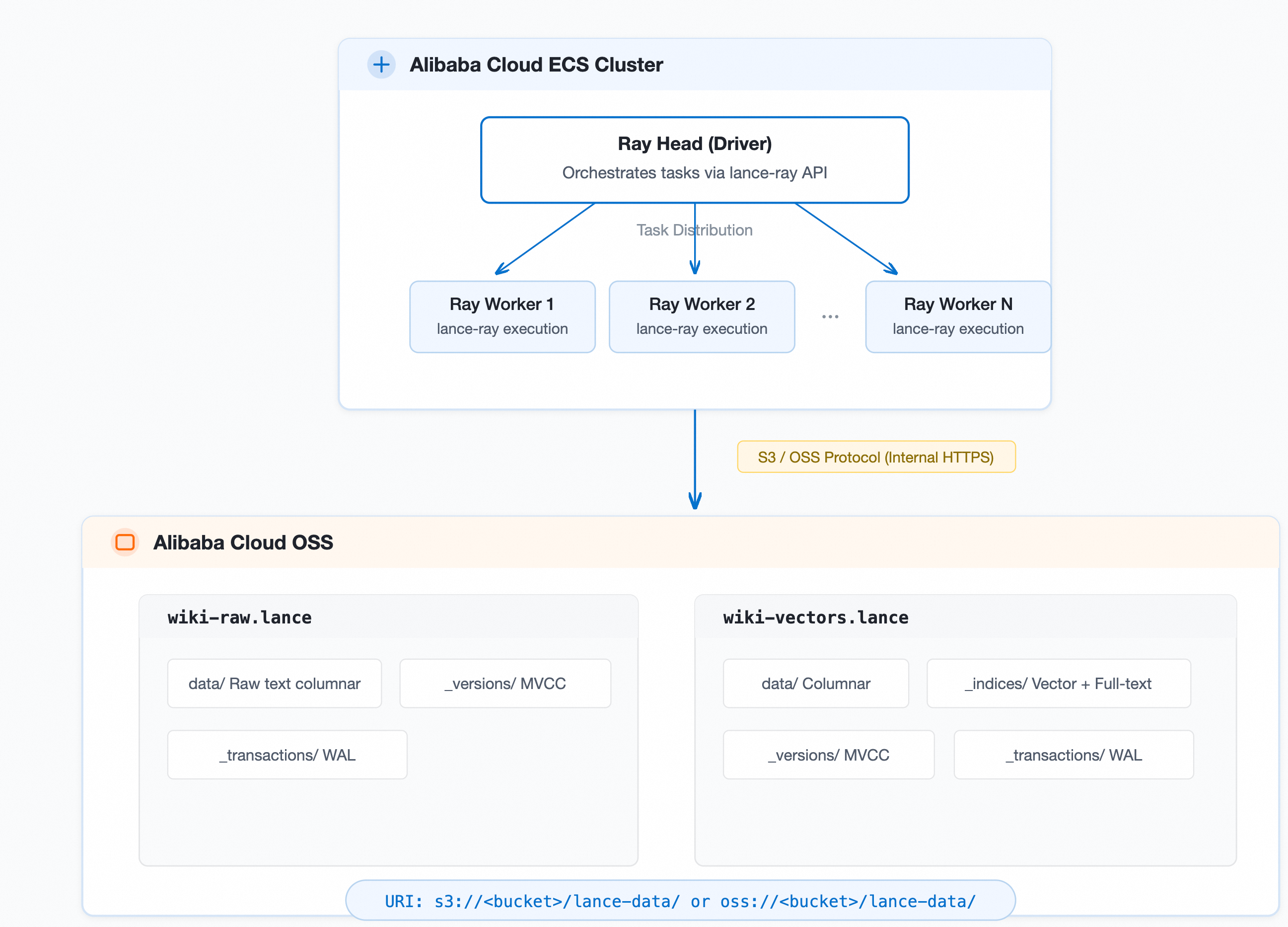
Data flow: Raw text → Write to OSS in Lance format → Distributed embedding on a Ray cluster → Write vector data back to OSS → Distributed index building → Vector, full-text, and hybrid search.

Prerequisites

• Alibaba Cloud ECS: We recommend three or more instances in the same availability zone (1 head + N workers). We suggest an instance type of 8-core 32 GB or higher, running Ubuntu 24.04 LTS.

• Alibaba Cloud OSS: Located in the same region as the ECS instances and accessed via an internal endpoint. For protocol configuration details, see Configure OSS as the Lance backend.

• Python 3.12 virtual environment, with the core dependencies installed:

  pip install "pylance>=6.0.0" "lance-ray>=0.4.2" "ray[data]>=2.41.0"
  pip install torch --index-url https://download.pytorch.org/whl/cpu
  pip install sentence-transformers "modelscope[framework]" datasets pandas pyarrow

• Ray cluster is ready:

  # Head node
  ray start --head --port=6379 --dashboard-host=0.0.0.0 --dashboard-port=8265
  
  # Worker node (pass the internal IP of the head)
  ray start --address=<HEAD_INTERNAL_IP>:6379

• OSS access credentials: Configure the access credentials as environment variables on the head node. Ray will automatically serialize and distribute them to the worker nodes.

  export BUCKET_NAME="<your-bucket-name>"
  
  # S3-compatible protocol (recommended, used by default in this tutorial)
  export AWS_ACCESS_KEY_ID="<your-access-key-id>"
  export AWS_SECRET_ACCESS_KEY="<your-access-key-secret>"
  export AWS_ENDPOINT="https://<bucket>.oss-cn-hangzhou-internal.aliyuncs.com"

Step 1: Prepare configuration

To make it easier to share parameters between steps, centralize all configurations in a config.py file, divided into storage and compute sections.

Storage configuration

This tutorial uses the S3-compatible protocol by default. For more details on the configuration principles, see Configure OSS as the Lance backend.

"""config.py — Storage configuration section"""

import os
from datetime import datetime

RUN_ID = os.environ.get("RUN_ID", datetime.now().strftime("%Y%m%d_%H%M%S"))

# Data volume (defined early, as write-tuning parameters depend on it)
NUM_SAMPLES = int(os.environ.get("NUM_SAMPLES", 100_000))

# OSS / Storage configuration (S3-compatible protocol)
BUCKET_NAME = os.environ["BUCKET_NAME"]
OSS_REGION = os.environ.get("OSS_REGION", "cn-hangzhou")

STORAGE_OPTIONS = {
    "region": OSS_REGION,
    "endpoint": os.environ.get(
        "AWS_ENDPOINT",
        f"https://{BUCKET_NAME}.oss-{OSS_REGION}-internal.aliyuncs.com",
    ),
    "access_key_id": os.environ["AWS_ACCESS_KEY_ID"],
    "secret_access_key": os.environ["AWS_SECRET_ACCESS_KEY"],
    "virtual_hosted_style_request": "true",
}

# Dataset URIs
RAW_DATASET_URI = f"s3://{BUCKET_NAME}/lance-data/{RUN_ID}/wiki-raw.lance"
VECTOR_DATASET_URI = f"s3://{BUCKET_NAME}/lance-data/{RUN_ID}/wiki-vectors.lance"

# Write tuning
RAW_MAX_ROWS_PER_FILE = min(NUM_SAMPLES, 100_000)
RAW_MIN_ROWS_PER_FILE = min(NUM_SAMPLES // 2, 50_000)
VECTOR_MAX_ROWS_PER_FILE = min(NUM_SAMPLES, 200_000)
VECTOR_MIN_ROWS_PER_FILE = min(NUM_SAMPLES // 2, 50_000)

Compute configuration

This includes the embedding model, Ray scheduling parameters, and index and search parameters. The Ray scheduling parameters are automatically inferred from the cluster topology by init_ray_config() after ray.init() is called.

"""config.py — Compute configuration section"""

import math

# Embedding model
EMBEDDING_MODEL = "sentence-transformers/all-MiniLM-L6-v2"
EMBEDDING_DIM = 384
TEXT_TRUNCATE_LENGTH = 512

# Ray parameters — auto-populated by init_ray_config()
RAY_CPUS_PER_WORKER = 2
RAY_NUM_WORKERS = None
RAY_MEMORY_PER_WORKER = None
ACTOR_MIN_SIZE = None
ACTOR_MAX_SIZE = None
RAY_REMOTE_ARGS = None

ENCODE_BATCH_SIZE = 256
MAP_BATCH_SIZE = 1024


def init_ray_config():
    """Called after ray.init() to automatically infer Ray scheduling parameters."""
    import ray

    global RAY_NUM_WORKERS, RAY_MEMORY_PER_WORKER
    global ACTOR_MIN_SIZE, ACTOR_MAX_SIZE, RAY_REMOTE_ARGS

    nodes = ray.nodes()
    alive_nodes = [n for n in nodes if n["Alive"]]
    num_nodes = len(alive_nodes)
    total_cpus = sum(n["Resources"].get("CPU", 0) for n in alive_nodes)
    total_memory_bytes = sum(n["Resources"].get("memory", 0) for n in alive_nodes)
    total_memory_gb = total_memory_bytes / 1024**3

    print(f"[config] Cluster: {num_nodes} nodes, "
          f"{total_cpus:.0f} CPUs, {total_memory_gb:.1f} GB schedulable memory")

    min_node_memory_gb = min(
        n["Resources"].get("memory", 0) for n in alive_nodes
    ) / 1024**3
    max_workers_per_node = max(1, int(min_node_memory_gb) // 10)
    RAY_MEMORY_PER_WORKER = int(
        min_node_memory_gb / max_workers_per_node * 0.8 * 1024**3
    )

    max_workers_by_cpu = int(total_cpus) // RAY_CPUS_PER_WORKER
    max_workers_by_mem = num_nodes * max_workers_per_node
    RAY_NUM_WORKERS = max(1, min(max_workers_by_cpu, max_workers_by_mem))

    ACTOR_MIN_SIZE = 2
    ACTOR_MAX_SIZE = min(6, max_workers_by_cpu)

    RAY_REMOTE_ARGS = {
        "num_cpus": RAY_CPUS_PER_WORKER,
        "memory": RAY_MEMORY_PER_WORKER,
    }

    print(f"[config] Auto-tuned: num_workers={RAY_NUM_WORKERS}, "
          f"memory/worker={RAY_MEMORY_PER_WORKER / 1024**3:.1f} GB, "
          f"actor_pool=[{ACTOR_MIN_SIZE}, {ACTOR_MAX_SIZE}]")


# Vector index
VECTOR_INDEX_NAME = "vector_idx"
VECTOR_INDEX_METRIC = "cosine"
IVF_NUM_PARTITIONS = max(16, min(4096, int(math.sqrt(NUM_SAMPLES))))
PQ_NUM_SUB_VECTORS = 48

# Full-text index
TITLE_FTS_INDEX_NAME = "title_fts_idx"
TEXT_FTS_INDEX_NAME = "text_fts_idx"
FTS_WITH_POSITION = True

# Search parameters
VECTOR_SEARCH_K = 10
KEYWORD_SEARCH_LIMIT = 20
HYBRID_VECTOR_K = 20
RRF_K = 60

# Data management
APPEND_BATCH_SIZE = min(10_000, NUM_SAMPLES // 10)

Step 2: Prepare raw data

Download the Wikipedia dataset from ModelScope and write it to OSS in the Lance format.

"""Step 2: Prepare the test dataset and write it to OSS in Lance format"""

import lance
import pyarrow as pa
from modelscope.msdatasets import MsDataset

from config import NUM_SAMPLES, RAW_DATASET_URI, RAW_MAX_ROWS_PER_FILE, STORAGE_OPTIONS


def main():
    print("Loading Wikipedia dataset from ModelScope...")
    ds = MsDataset.load(
        "wikimedia/wikipedia",
        subset_name="20231101.en",
        split=f"train[:{NUM_SAMPLES}]",
        trust_remote_code=True,
    )

    print(f"Loaded {len(ds)} articles")
    print(f"Sample: {ds[0]['title']}")

    table = pa.table(
        {
            "doc_id": pa.array(range(len(ds)), type=pa.int64()),
            "title": pa.array(ds["title"], type=pa.utf8()),
            "text": pa.array(ds["text"], type=pa.utf8()),
        }
    )

    print(f"Writing {table.num_rows} rows to OSS: {RAW_DATASET_URI}")

    lance.write_dataset(
        table,
        RAW_DATASET_URI,
        storage_options=STORAGE_OPTIONS,
        max_rows_per_file=RAW_MAX_ROWS_PER_FILE,
    )

    ds_lance = lance.dataset(RAW_DATASET_URI, storage_options=STORAGE_OPTIONS)
    print("Dataset written successfully!")
    print(f"  Rows: {ds_lance.count_rows()}")
    print(f"  Fragments: {len(ds_lance.get_fragments())}")
    print(f"  Schema: {ds_lance.schema}")
    print(f"  Version: {ds_lance.version}")


if __name__ == "__main__":
    main()

Step 3: Generate distributed embeddings

Distribute the embedding computation across multiple nodes in the cluster using a Ray Actor Pool. Each Actor loads the model instance once and processes multiple batches, avoiding the overhead of reloading the model repeatedly. The entire pipeline streams data in blocks between the read → compute → write stages, eliminating the need to load the entire dataset before processing.

"""Step 3: Use Ray to generate embedding vectors in a distributed manner and write them back to OSS in Lance format"""

import time

import lance
import lance_ray as lr
import ray

import config
from config import (
    EMBEDDING_MODEL,
    ENCODE_BATCH_SIZE,
    MAP_BATCH_SIZE,
    RAW_DATASET_URI,
    RAY_CPUS_PER_WORKER,
    STORAGE_OPTIONS,
    TEXT_TRUNCATE_LENGTH,
    VECTOR_DATASET_URI,
    VECTOR_MAX_ROWS_PER_FILE,
    VECTOR_MIN_ROWS_PER_FILE,
    init_ray_config,
)


class EmbeddingGenerator:
    """Ray Actor: Loads the model once per worker to process multiple batches"""

    def __init__(self):
        from modelscope import snapshot_download
        from sentence_transformers import SentenceTransformer

        local_path = snapshot_download(EMBEDDING_MODEL)
        self.model = SentenceTransformer(local_path)
        print(f"Model loaded on worker: {EMBEDDING_MODEL}")

    def __call__(self, batch: dict) -> dict:
        texts = [
            f"{title}: {text[:TEXT_TRUNCATE_LENGTH]}"
            for title, text in zip(batch["title"], batch["text"])
        ]

        embeddings = self.model.encode(
            texts,
            batch_size=ENCODE_BATCH_SIZE,
            show_progress_bar=False,
            normalize_embeddings=True,
        )

        import numpy as np
        import pyarrow as pa

        flat = embeddings.astype(np.float32).ravel()
        batch["vector"] = pa.FixedSizeListArray.from_arrays(
            pa.array(flat, type=pa.float32()),
            list_size=embeddings.shape[1],
        )
        return batch


def main():
    ray.init(address="auto")
    init_ray_config()

    print("\n=== Phase 1: Reading raw data from OSS ===")
    t0 = time.time()

    ds = lr.read_lance(
        RAW_DATASET_URI,
        columns=["doc_id", "title", "text"],
        storage_options=STORAGE_OPTIONS,
    )

    print(f"Read dataset: {ds.count()} rows, took {time.time()-t0:.1f}s")
    print(f"Schema: {ds.schema()}")

    print("\n=== Phase 2: Distributed Embedding Generation ===")
    t1 = time.time()

    ds_with_vectors = ds.map_batches(
        EmbeddingGenerator,
        batch_size=MAP_BATCH_SIZE,
        compute=ray.data.ActorPoolStrategy(
            min_size=config.ACTOR_MIN_SIZE,
            max_size=config.ACTOR_MAX_SIZE,
        ),
        num_gpus=0,
        num_cpus=RAY_CPUS_PER_WORKER,
    )

    print(f"Embedding generation configured, took {time.time()-t1:.1f}s to plan")

    print("\n=== Phase 3: Writing vectors to OSS in Lance format ===")
    t2 = time.time()

    lr.write_lance(
        ds_with_vectors,
        VECTOR_DATASET_URI,
        storage_options=STORAGE_OPTIONS,
        mode="create",
        max_rows_per_file=VECTOR_MAX_ROWS_PER_FILE,
        min_rows_per_file=VECTOR_MIN_ROWS_PER_FILE,
    )

    write_time = time.time() - t2
    print(f"Write completed in {write_time:.1f}s")

    print("\n=== Verification ===")
    result_ds = lance.dataset(VECTOR_DATASET_URI, storage_options=STORAGE_OPTIONS)
    print(f"Total rows: {result_ds.count_rows()}")
    print(f"Fragments: {len(result_ds.get_fragments())}")
    print(f"Schema: {result_ds.schema}")
    print(f"Dataset version: {result_ds.version}")

    sample = result_ds.take(indices=[0])
    print(f"Sample doc_id: {sample['doc_id'][0].as_py()}")
    print(f"Sample title: {sample['title'][0].as_py()}")
    print(f"Sample vector dim: {len(sample['vector'][0].as_py())}")
    print(f"Sample vector[:5]: {sample['vector'][0].as_py()[:5]}")

    total_time = time.time() - t0
    print(f"\nTotal pipeline time: {total_time:.1f}s")

    ray.shutdown()


if __name__ == "__main__":
    main()

Step 4: Build distributed index and run ANN search

Use lance-ray to build an IVF_PQ vector index in a distributed manner. The index data is written directly to the Lance dataset directory on OSS, without needing intermediate local disk storage.

"""Step 4: Use Ray to build an IVF_PQ vector index in a distributed manner"""

import time

import lance
import lance_ray as lr
import ray

import config
from config import (
    IVF_NUM_PARTITIONS,
    PQ_NUM_SUB_VECTORS,
    STORAGE_OPTIONS,
    VECTOR_DATASET_URI,
    VECTOR_INDEX_METRIC,
    VECTOR_INDEX_NAME,
    VECTOR_SEARCH_K,
    init_ray_config,
)


def main():
    ray.init(address="auto")
    init_ray_config()

    ds = lance.dataset(VECTOR_DATASET_URI, storage_options=STORAGE_OPTIONS)
    num_rows = ds.count_rows()
    num_fragments = len(ds.get_fragments())
    print(f"Dataset: {num_rows} rows, {num_fragments} fragments")

    print("\n=== Building IVF_PQ Vector Index ===")
    print(f"  num_partitions={IVF_NUM_PARTITIONS}, num_sub_vectors={PQ_NUM_SUB_VECTORS}")
    t0 = time.time()

    updated_ds = lr.create_index(
        VECTOR_DATASET_URI,
        column="vector",
        index_type="IVF_PQ",
        name=VECTOR_INDEX_NAME,
        metric=VECTOR_INDEX_METRIC,
        num_partitions=IVF_NUM_PARTITIONS,
        num_sub_vectors=PQ_NUM_SUB_VECTORS,
        num_workers=config.RAY_NUM_WORKERS,
        storage_options=STORAGE_OPTIONS,
        ray_remote_args=config.RAY_REMOTE_ARGS,
    )

    index_time = time.time() - t0
    print(f"Vector index built in {index_time:.1f}s")

    indices = updated_ds.list_indices()
    print(f"Indices: {indices}")
    print(f"Dataset version after indexing: {updated_ds.version}")

    print("\n=== Testing ANN Search ===")

    sample = updated_ds.take(indices=[42])
    query_vector = sample["vector"][0].as_py()
    query_title = sample["title"][0].as_py()
    print(f"Query document: '{query_title}'")

    t1 = time.time()
    results = updated_ds.to_table(
        nearest={"column": "vector", "q": query_vector, "k": VECTOR_SEARCH_K},
        columns=["doc_id", "title"],
    )
    search_time = time.time() - t1
    print(
        f"ANN search completed in {search_time*1000:.1f}ms, "
        f"found {results.num_rows} results:"
    )

    for i in range(results.num_rows):
        doc_id = results.column("doc_id")[i].as_py()
        title = results.column("title")[i].as_py()
        print(f"  [{i+1}] doc_id={doc_id}, title='{title}'")

    ray.shutdown()


if __name__ == "__main__":
    main()

Step 5: Build full-text index and run hybrid search

Build an inverted index (INVERTED) in a distributed manner and combine it with vector search to implement hybrid search. This approach uses Reciprocal Rank Fusion (RRF) to merge the results from both retrieval methods, balancing semantic similarity with keyword matching.

"""Step 5: Build a full-text index and perform a hybrid search (vector + keyword)"""

import time

import lance
import lance_ray as lr
import ray

import config
from config import (
    EMBEDDING_MODEL,
    FTS_WITH_POSITION,
    HYBRID_VECTOR_K,
    KEYWORD_SEARCH_LIMIT,
    RRF_K,
    STORAGE_OPTIONS,
    TEXT_FTS_INDEX_NAME,
    TITLE_FTS_INDEX_NAME,
    VECTOR_DATASET_URI,
    VECTOR_SEARCH_K,
    init_ray_config,
)


def main():
    ray.init(address="auto")
    init_ray_config()

    # Build an inverted index in a distributed manner
    print("=== Building Full-Text Index ===")
    t0 = time.time()

    lr.create_scalar_index(
        VECTOR_DATASET_URI,
        column="title",
        index_type="INVERTED",
        name=TITLE_FTS_INDEX_NAME,
        num_workers=config.RAY_NUM_WORKERS,
        storage_options=STORAGE_OPTIONS,
        ray_remote_args=config.RAY_REMOTE_ARGS,
        with_position=FTS_WITH_POSITION,
    )

    fts_time = time.time() - t0
    print(f"Full-text index on 'title' built in {fts_time:.1f}s")

    print("\nBuilding FTS index on 'text' column...")
    t1 = time.time()

    lr.create_scalar_index(
        VECTOR_DATASET_URI,
        column="text",
        index_type="INVERTED",
        name=TEXT_FTS_INDEX_NAME,
        num_workers=config.RAY_NUM_WORKERS,
        storage_options=STORAGE_OPTIONS,
        ray_remote_args=config.RAY_REMOTE_ARGS,
        with_position=FTS_WITH_POSITION,
    )

    print(f"Text FTS index built in {time.time()-t1:.1f}s")

    ds = lance.dataset(VECTOR_DATASET_URI, storage_options=STORAGE_OPTIONS)
    print(f"\nAll indices: {ds.list_indices()}")

    # Full-text search
    print("\n=== Full-Text Search ===")

    query_text = "machine learning neural network"
    t2 = time.time()

    fts_results = ds.to_table(
        full_text_query=query_text,
        columns=["doc_id", "title"],
        limit=VECTOR_SEARCH_K,
    )

    fts_search_time = time.time() - t2
    print(f"FTS query '{query_text}' completed in {fts_search_time*1000:.1f}ms")
    print(f"Found {fts_results.num_rows} results:")
    for i in range(min(5, fts_results.num_rows)):
        print(f"  [{i+1}] {fts_results.column('title')[i].as_py()}")

    # Hybrid search (vector + full-text)
    print("\n=== Hybrid Search (Vector + Full-Text) ===")

    user_question = "What are the applications of deep learning in healthcare?"

    from modelscope import snapshot_download
    from sentence_transformers import SentenceTransformer

    local_path = snapshot_download(EMBEDDING_MODEL)
    model = SentenceTransformer(local_path)
    query_vector = model.encode(user_question, normalize_embeddings=True).tolist()

    t3 = time.time()
    vector_results = ds.to_table(
        nearest={"column": "vector", "q": query_vector, "k": HYBRID_VECTOR_K},
        columns=["doc_id", "title", "text"],
    )
    vector_time = time.time() - t3

    t4 = time.time()
    keyword_results = ds.to_table(
        full_text_query="deep learning healthcare",
        columns=["doc_id", "title", "text"],
        limit=KEYWORD_SEARCH_LIMIT,
    )
    keyword_time = time.time() - t4

    print(f"\nUser question: '{user_question}'")
    print(
        f"Vector search: {vector_results.num_rows} results in {vector_time*1000:.1f}ms"
    )
    print(
        f"Keyword search: {keyword_results.num_rows} results in {keyword_time*1000:.1f}ms"
    )

    # Reciprocal Rank Fusion
    doc_scores = {}
    doc_titles = {}

    for i in range(vector_results.num_rows):
        doc_id = vector_results.column("doc_id")[i].as_py()
        doc_scores[doc_id] = doc_scores.get(doc_id, 0) + 1.0 / (RRF_K + i)
        doc_titles[doc_id] = vector_results.column("title")[i].as_py()

    for i in range(keyword_results.num_rows):
        doc_id = keyword_results.column("doc_id")[i].as_py()
        doc_scores[doc_id] = doc_scores.get(doc_id, 0) + 1.0 / (RRF_K + i)
        doc_titles[doc_id] = keyword_results.column("title")[i].as_py()

    ranked_docs = sorted(doc_scores.items(), key=lambda x: x[1], reverse=True)[:10]

    print("\nHybrid search top results (RRF fusion):")
    for rank, (doc_id, score) in enumerate(ranked_docs, 1):
        title = doc_titles.get(doc_id, "Unknown")
        print(f"  [{rank}] score={score:.4f} | {title}")

    ray.shutdown()


if __name__ == "__main__":
    main()

Step 6: Maintain data: Appends, compaction, and versioning

This section demonstrates common data maintenance operations in a production environment: incremental appends, distributed compaction, and version-based time travel.

"""Step 6: Data management — Incremental appends, distributed compaction, and version management"""

import time

import lance
import lance_ray as lr
import numpy as np
import pyarrow as pa
import ray
from lance_ray.compaction import CompactionOptions

import config
from config import (
    APPEND_BATCH_SIZE,
    EMBEDDING_DIM,
    STORAGE_OPTIONS,
    VECTOR_DATASET_URI,
    init_ray_config,
)


def main():
    ray.init(address="auto")
    init_ray_config()

    ds = lance.dataset(VECTOR_DATASET_URI, storage_options=STORAGE_OPTIONS)
    print(f"Current state: {ds.count_rows()} rows, {len(ds.get_fragments())} fragments")
    print(f"Current version: {ds.version}")

    # 1. Incremental append (This example uses random vectors. In production, you should use an embedding model to generate real vectors.)
    print("\n=== Incremental Append ===")

    num_new = APPEND_BATCH_SIZE
    start_id = ds.count_rows()
    new_docs = pa.table(
        {
            "doc_id": pa.array(
                range(start_id, start_id + num_new), type=pa.int64()
            ),
            "title": pa.array(
                [f"New Document {i}" for i in range(num_new)], type=pa.utf8()
            ),
            "text": pa.array(
                [
                    f"This is new content for document {i}. Updated knowledge base entry."
                    for i in range(num_new)
                ],
                type=pa.utf8(),
            ),
            "vector": pa.FixedSizeListArray.from_arrays(
                pa.array(
                    (lambda v: (v / np.linalg.norm(v, axis=1, keepdims=True)).ravel())(
                        np.random.randn(num_new, EMBEDDING_DIM).astype(np.float32)
                    )
                ),
                list_size=EMBEDDING_DIM,
            ),
        }
    )

    ray_ds = ray.data.from_arrow(new_docs)
    lr.write_lance(
        ray_ds,
        VECTOR_DATASET_URI,
        storage_options=STORAGE_OPTIONS,
        mode="append",
    )

    ds_after_append = lance.dataset(VECTOR_DATASET_URI, storage_options=STORAGE_OPTIONS)
    print(
        f"After append: {ds_after_append.count_rows()} rows, "
        f"{len(ds_after_append.get_fragments())} fragments"
    )
    print(f"New version: {ds_after_append.version}")

    # 2. Distributed compaction
    print("\n=== Distributed Compaction ===")

    t0 = time.time()
    metrics = lr.compact_files(
        VECTOR_DATASET_URI,
        compaction_options=CompactionOptions(),
        num_workers=config.RAY_NUM_WORKERS,
        storage_options=STORAGE_OPTIONS,
        ray_remote_args=config.RAY_REMOTE_ARGS,
    )
    compact_time = time.time() - t0

    if metrics:
        print(f"Compaction completed in {compact_time:.1f}s")
        print(f"Metrics: {metrics}")
    else:
        print("No compaction needed")

    ds_after_compact = lance.dataset(
        VECTOR_DATASET_URI, storage_options=STORAGE_OPTIONS
    )
    print(
        f"After compaction: {ds_after_compact.count_rows()} rows, "
        f"{len(ds_after_compact.get_fragments())} fragments"
    )

    # 3. Version management (time travel)
    print("\n=== Version Management (Time Travel) ===")

    versions = ds_after_compact.versions()
    print(f"Total versions: {len(versions)}")
    for v in versions[-3:]:
        print(f"  Version {v['version']}: {v['timestamp']}")

    old_version = versions[0]["version"]
    ds_old = lance.dataset(
        VECTOR_DATASET_URI,
        version=old_version,
        storage_options=STORAGE_OPTIONS,
    )
    print(f"\nOld version ({old_version}): {ds_old.count_rows()} rows")
    print(
        f"Current version ({ds_after_compact.version}): "
        f"{ds_after_compact.count_rows()} rows"
    )

    ray.shutdown()


if __name__ == "__main__":
    main()

Results

These results are from a 3-node Ray cluster (3 × 8-core, 32 GB ECS instances) processing 100,000 Wikipedia documents.

Performance benchmarks

Search results

ANN vector search — Using "Crouching Tiger, Hidden Dragon" as the query vector to search for the most semantically similar documents directly on OSS:

Query: 'Crouching Tiger, Hidden Dragon'

  [1] Crouching Tiger, Hidden Dragon
  [2] Cheng Pei-pei
  [3] Dragon Lord
  [4] Dragon Fist (manga)
  [5] The White Dragon (film)
  [6] Tiger Child
  [7] Wu Yonggang
  [8] Sam Lee (actor)
  [9] Action of the Tiger
  [10] New Fist of Fury

Hybrid search — For the user question "What are the applications of deep learning in healthcare?", the system performs both a vector semantic search and a keyword full-text search, then fuses the results with RRF:

User question: 'What are the applications of deep learning in healthcare?'

Vector search:  20 results in ~1265ms
Keyword search: 20 results in ~347ms

Hybrid top results (RRF fusion):
  [1] List of artificial intelligence projects
  [2] Predictive analytics
  [3] Artificial intelligence
  [4] Clinical engineering
  [5] NeuroSolutions

Version management and time travel

Lance uses an MVCC mechanism to implement zero-copy snapshots on OSS. Every write operation (append, index building, compaction) automatically creates a new version. New and old versions share unchanged data files, resulting in almost no extra storage overhead:

Total versions: 7

Version 1: 100,000 rows  ← Initial write
Version 4: 100,000 rows  ← After index building
Version 5: 110,000 rows  ← Incremental append of 10,000 rows
Version 7: 110,000 rows  ← After compaction

# Time travel: Roll back to any historical version at any time
ds_old = lance.dataset(uri, version=1)  → 100,000 rows
ds_new = lance.dataset(uri, version=7)  → 110,000 rows

Advanced: Accelerate RAG retrieval with OSS Accelerator

After completing the previous steps, the dataset is ready for online retrieval. In a production RAG system, retrieval latency directly impacts user experience and system throughput. This section validates the performance improvement of using the OSS Accelerator for online retrieval with Lance.

Online retrieval in Lance (vector, full-text, or hybrid search) is essentially a series of high-frequency random reads of index and data files on OSS. For example, a single vector search needs to read multiple partitions of an IVF index. If Product Quantization (PQ) refinement is enabled, it also needs to read the original vectors for re-ranking. This I/O latency directly limits retrieval performance. The OSS Accelerator provides a low-latency, high-throughput data path between compute nodes and OSS, significantly reducing the time for each I/O operation. Moreover, Lance's "write, then read repeatedly" or read-after-write pattern is a natural fit for the accelerator's synchronous warming feature. Data is cached during the writing phase, eliminating the need for an extra pre-warming step.

Test scenario

Based on the Wikipedia vector knowledge base built in the preceding pipeline, we simulate a real-world, end-to-end RAG online retrieval process: input text query → embedding inference → OSS retrieval → return results. We used a 6-node Ray cluster and a dataset of 100,000 documents (with a 316-partition IVF_PQ vector index and a full-text inverted index). 36 concurrent workers independently executed the complete retrieval process, initiating 5,000 retrieval requests for each scenario. The test ran under steady-state conditions after a service warm-up.

Accelerator configuration

The OSS Accelerator used in this test was enabled through the Alibaba Cloud console with the following configuration:

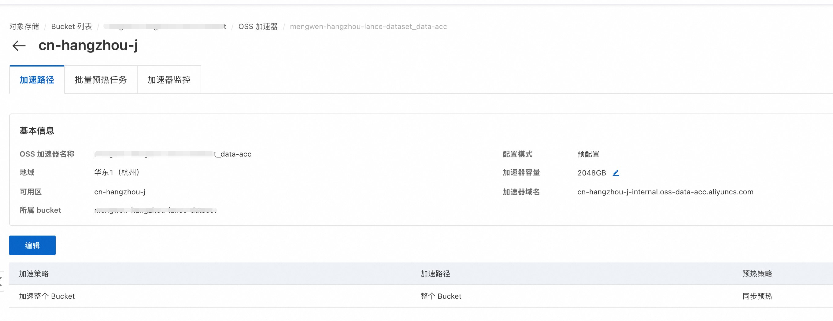
No changes are needed in the application code. Simply replace the endpoint in storage_options with the accelerator's address to activate it.

Test parameters

Test results

The following tables compare the performance of standard OSS and OSS Accelerator in an end-to-end RAG scenario.

Total task time comparison (5,000 requests, 36 concurrent workers, steady state):

Retrieval latency comparison (p50 median):

Key conclusions

• Total task time is halved: The time to complete 5,000 vector searches decreased from 15.4s to 7.8s (2.0x speedup), and hybrid searches from 26.2s to 13.0s (2.0x speedup).

• Median (p50) retrieval-only latency is reduced by 2.7x to 2.8x: Vector search latency dropped from 85.5ms to 30.2ms (2.8x speedup), and hybrid search latency from 161.5ms to 60.2ms (2.7x speedup).

Production best practices

Storage access configuration

• Prioritize the S3-compatible protocol: Its mature ecosystem and conditional write semantics are unaffected by the bucket's versioning status, making it suitable for multi-writer concurrency in production. For configuration details, see Configure OSS as the Lance backend.

• Use an internal endpoint: When your ECS instances and OSS bucket are in the same region, use an internal endpoint for higher bandwidth and no data transfer fees.

Online retrieval acceleration

• Enable OSS Accelerator: For high-frequency random read scenarios like Lance vector and full-text search, the OSS Accelerator can reduce retrieval-only latency by 2.7x to 2.8x and improve overall throughput by 2.0x. Activating it is as simple as switching the endpoint to the accelerator's address, with no code changes required.

• Automatic warming with read-after-write: Data is cached by the accelerator during the writing and index-building phases. Subsequent retrieval requests are served directly from the cache, eliminating the need for a separate warm-up process.

Cost optimization

• Storage-compute separation: By storing data in OSS, compute nodes do not require data disks and can be elastically scaled on a pay-as-you-go basis.

• Zero-copy versions and version cleanup: Lance's MVCC ensures that new and old versions share unchanged data files, so version snapshots incur almost no extra storage cost. When cleaning up old versions, you must use the Lance API. Do not rely on external storage lifecycle policies, which can cause the accidental deletion of shared files that are still referenced by the current version:

  # Clean up old versions and their unreferenced data files older than 7 days
  from datetime import timedelta
  ds = lance.dataset(uri, storage_options=storage_options)
  ds.cleanup_old_versions(older_than=timedelta(days=7))

Ray distributed tuning

• Automatic resource discovery: After calling ray.init(), call init_ray_config() to automatically infer the number of workers, memory allocation, and Actor Pool size from the cluster topology.

• Fragments as the unit of parallelism: lance-ray assigns index-building tasks on a per-fragment basis. You can control the number of fragments with max_rows_per_file during the write phase. The number of fragments determines the maximum parallelism for index building.

• Elastic Actor Pool and pipeline backpressure: During the embedding stage, use ActorPoolStrategy(min_size, max_size) to allow Ray to automatically scale the number of model instances based on the load. Ray Data's streaming pipeline has a built-in backpressure mechanism that automatically coordinates the rates of the read, compute, and write stages. You can monitor operator throughput and backlogs in the Ray Data panel of the Ray Dashboard.