Industrial background
Road traffic scheduling aims to achieve efficient operation and flow control for a transportation system by properly managing and scheduling transportation resources. How can scheduling be arranged to help improve transportation efficiency and reduce costs? This optimization problem can be modeled and solved using mathematical programming methods.
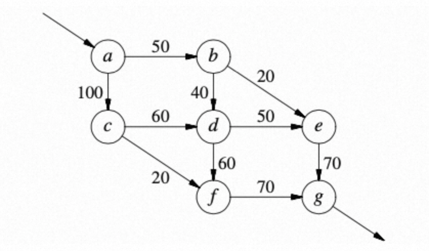
For example, there are seven stations, and each station has several entry roads and exit roads. The number beside a road indicates the maximum number of vehicles that this road can carry in unit time. How can vehicles be scheduled to obtain the maximum number of vehicles that depart from station a and finally arrive at station g per unit time?
Business research, data quantification, and mathematical modeling
When using optimization techniques, you need to investigate the needs of business in more detail, organize the relevant business logic and data, and quantify them. Then, you can use a mathematical programming method for modeling.
For more details, see . This section lists only the related mathematical formula.

In this formula, i represents the starting point of a road, j represents the destination of the road, e represents the origin station, k represents an intermediate station, and r represents the number of vehicles that can pass.
Constraints on the preceding formula:
The number of vehicles that enter an intermediate station is equal to the number of vehicles that leave the station.
A limited number of vehicles can pass through each channel.
Source code
You can call MindOpt from various programming or modeling languages. The following is an example:
Calling the MindOpt APL modeling language
Source code for MindOpt APL (you can access to perform a dry run):
##====Source code for MindOpt APL====

clear model;

# Modeling
# net1.mapl
set Station :={"a","b","c","d","e","f","g"};
set Middle := {"b","c","d","e","f"};
set Roads :={<"a","b">,<"b","d">,<"c","d">,<"d","e">,<"e","g">,<"a","c">,<"b","e">,<"c","f">,<"d","f">,<"f","g">};

param entr := "a";

param lb := 0;
param ub[Roads] := <"a","b"> 50, <"b","d"> 40, <"c","d"> 60, <"d","e"> 50, <"e","g"> 70, <"a","c"> 100, <"b","e"> 20, <"c","f"> 20, <"d","f"> 60, <"f","g"> 70;

var x[<i,j> in Roads] >= lb <= ub[i,j];

maximize Total : sum {<entr,j> in Roads } x[entr,j]; # The maximum inbound traffic at a start station.

# Traffic balancing
subto Balance:
    forall <k> in Middle do
        sum {<i,k> in Roads} x[i,k] == sum {<k,j> in Roads } x[k,j];


print "------------- Solving using Optimization Solver---------------";
option solver mindopt; # (Optional) Specifies the solver used for solving the problem. Optimization Solver is used by default.
#option mindopt_options 'print=0'; # Sets output levels for the solver to simplify outputs.
solve; # Solves the problem.

print "----------------- Result ---------------";
display; # Displays the result.
print "Maximum road traffic after optimization = " ,sum {<entr,j> in Roads } x[entr,j];
Result and result usage
The logs vary based on code. The following section provides a part of the logs.
...
Model summary.
 - Num. variables     : 10
 - Num. constraints   : 5
 - Num. nonzeros      : 16
 - Bound range        : [2.0e+01,1.0e+02]
 - Objective range    : [1.0e+00,1.0e+00]
 - Matrix range       : [1.0e+00,1.0e+00]
...
Simplex method terminated. Time : 0.002s


OPTIMAL; objective 130.00
...
----------------- Result ---------------
Maximum road traffic after optimization = 130
The optimal solution is 130. If you want to learn more details of the solution, such as the values of the decision variables and whether the constraints are correct, you can run the print command or obtain the values of the decision variables from the .sol file for programming. You can also run the display command to obtain the values of all variables.
For example, run the following command to verify the constraint that the number of vehicles that enter an intermediate station is equal to the number of vehicles that leave the station.
forall <k> in Middle do
  print 'Number of vehicles entering station {}: {}'%k, sum {<i,k> in Roads} x[i,k];
print "-------------";
forall <k> in Middle do
  print 'Number of vehicles leaving station {}: {}'%k, sum {<k,j> in Roads} x[k,j];
The following outputs are equivalent:
Number of vehicles entering station b:50
Number of vehicles entering station c:80
Number of vehicles entering station d:90
Number of vehicles entering station e:70
Number of vehicles entering station f:60
-------------
Number of vehicles leaving station b:50
Number of vehicles leaving station c:80
Number of vehicles leaving station d:90
Number of vehicles leaving station e:70
Number of vehicles leaving station f:60
Run the following code to display the results in CSV format as a solution to the road traffic scheduling problem:
print "{},{},{} "% "Start station","Intermediate station","Number of vehicles" : "Results.csv";
close "Results.csv";

forall {<i,j> in Roads}
    print "{},{},{}" % i,j,x[i,j]  >> "Results.csv";

close "Results.csv";
The output is as follows:
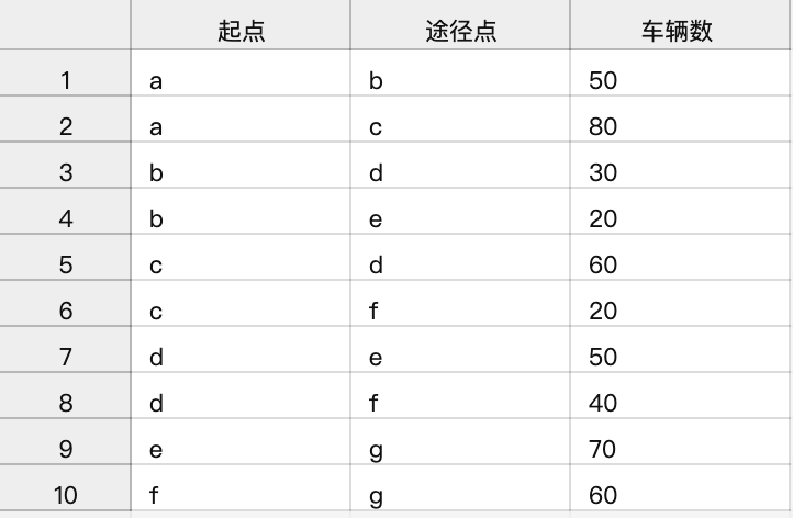
This means a maximum of 130 vehicles can depart from station a. The traffic is split as shown in the following figure.
The distance from a to b is 50, and the distance from a to c is 80.
The distance from b to d is 30, and from b to e is 20.
The path from c to d is 60, and the path from c to f is 20.
d aggregates a traffic volume of 90 and diverts 50 to e and 40 to f.
It aggregated 70% of the traffic
f aggregates a traffic volume of 60, which is then aggregated at exit g, resulting in a total of 130.