Problems in production scheduling and planning can also be modeled by using mathematical programming and solved by calling Optimization Solver.
Industrial background
Production scheduling and planning, raw material procurement, and warehousing are the key issues for the manufacturing industry to reduce costs and increase efficiency. How can the purchase amount of raw materials and production plan be reasonably scheduled to minimize costs or maximize profits? This optimization problem can also be modeled and solved by using mathematical programming methods.
For example, a soap manufacturer needs to plan for the soap production and raw material procurement in the next six months. Raw materials must be reserved in advance, but warehousing incurs costs. The procurement of raw materials needs to be scheduled as reasonably as possible so that an appropriate level of stock is maintained to ensure production.
Business research, data quantification, and mathematical modeling
When using optimization techniques, you need to investigate the needs of business in more detail, organize the relevant business logic and data, and quantify them. Then, you can use a mathematical programming method for modeling.
For more details, see the case Production Scheduling and Planning. This section lists only the mathematical formula.
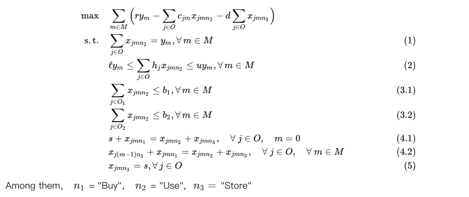
In the preceding formula, set O represents oil, which is denoted as O1 and O2, and M represents months.
Constraints on the preceding formula:
Oil is not wasted when it is made into soap. That is, weight is conserved in the production process.
The conversion of hardness in the production process from oil to soap follows a linear relationship.
The sum of the oil storage quantity in the previous month and the purchase quantity in the current month must equal the sum of the usage quantity and the storage quantity in the current month.
 is the initial storage quantity for each type of oil in January.
The total purchase quantities of vegetable oil and animal oil are limited.
The storage quantity for each type of oil at the end of June must be equal to the initial storage quantity for each type of oil in early January.
Source code
Optimization Solver supports multiple programming languages or modeling languages. This section provides only one of the languages for reference.
MindOpt APL
Source code for MindOpt Algebra Programming Language (MindOpt APL) (you can perform a trial run of the code in Production Scheduling and Planning):
##====Source code for MindOpt APL====

clear model;# Clear the model, which is used when you run the code multiple times.
option modelname manufacture_03_soap2;

# --------- Modeling -----------------
# manufacture_03_soap2.mapl

# Sets
set O1 := { "VEG1", "VEG2" };
set O2 := {"OIL1", "OIL2", "OIL3"};
set O :=  O1 + O2;
set M := {1, 2, 3, 4, 5, 6};
set N := {"Buy", "Use", "Store"};

# Parameters
param cost[O * M] :=
       |    1,     2,     3,     4,     5,    6    |
|"VEG1"|  110,   130,   110,   120,   100,   90    |
|"VEG2"|  120,   130,   140,   110,   120,   100   |
|"OIL1"|  130,   110,   130,   120,   150,   140   |
|"OIL2"|  110,    90,   100,   120,   110,   80    |
|"OIL3"|  115,   115,    95,   125,   105,   135   |;

param hardness[O] := <"VEG1"> 8.0, <"VEG2"> 6.0,
                     <"OIL1"> 2.0, <"OIL2"> 4.0, <"OIL3"> 5.0;

param r  := 150;
param b1 := 200;
param b2 := 250;
param l  := 3;
param u  := 6;
param s  := 500;
param d  := 5;

# Variables
var x[O * M * N] >= 0;
var y[M] >= 0;

# Objective
maximize Reward:  sum {<m> in M}(
                            r * y[m]
                                - sum {<j> in O} cost[j, m] * x[j, m, "Buy"]
                                - d * sum{<j> in O} x[j, m, "Store"]
                                );

# Constraints
subto Weight:
    forall { <m> in M }
        sum {<j> in O} x[j, m, "Use"] == y[m];

subto Hardness1:
    forall { <m> in M }
        sum {<j> in O} hardness[j] * x[j, m, "Use"] >= y[m] * l;

subto Hardness2:
    forall {<m> in M }
        sum {<j> in O} hardness[j] * x[j, m, "Use"] <= y[m] * u;

subto VEGBound:
    forall {<m> in M }
        sum {<j> in O1} x[j, m, "Use"] <= b1;

subto OILBound:
    forall { <m> in M }
        sum {<j> in O2} x[j, m, "Use"] <= b2;

subto Link_1:
    forall {<j, 1> in O * M }
        s + x[j,1,"Buy"] == x[j,1,"Use"] + x[j,1,"Store"];

subto Link_2to6:
    forall {<j, m> in O * M with m > 1 }
        x[j,m-1,"Store"] + x[j,m,"Buy"] == x[j,m,"Use"] + x[j,m,"Store"];

subto Store_June:
    forall { <j> in O }
        x[j,6,"Store"] == s;

#------------------------------

print "------------- Solving by using Optimization Solver---------------";
option solver mindopt; # Specify Optimization Solver for solving the problem.
solve; # Solving
# display; # Print variable values. This process takes a long time. Uncomment it before print.

print "----------------- Result ---------------";
print "Maximum profit= ", sum {<m> in M}(
                    r * y[m]
                        - sum {<j> in O} cost[j, m] * x[j, m, "Buy"]
                        - d * sum{<j> in O} x[j, m, "Store"]
                    );
Solution and use of the result
The logs vary based on code. The following section provides a part of logs.
...
Model summary.
 - Num. variables : 96
 - Num. constraints : 60
 - Num. nonzeros : 253
 - Bound range : [2.0e+02,5.0e+02]
 - Objective range : [5.0e+00,1.5e+02]
 - Matrix range : [1.0e+00,8.0e+00]
...
Simplex method terminated. Time : 0.002s
...
OPTIMAL; objective 108250.00
...
----------------- Result ---------------
Maximum profit = 108250
The optimal solution is 108250. If you want to learn more details of the solution, such as the value of the decision variable, you can run the print command or obtain them from the .sol file for programming. You can also run the display command to obtain the values of all variables.
Run the following command to verify the constraint that the storage quantity for each type of oil at the end of June must be equal to the initial storage quantity for each type of oil in early January:
forall {<j> in O} print 'Storage quantity at the end of June (',j,') = ', x[j,6,"Store"];The solution is 500, which is the same as the need in early January.
Storage quantity at the end of June (VEG1) = 500
Storage quantity at the end of June (VEG2) = 500
Storage quantity at the end of June (OIL1) = 500
Storage quantity at the end of June (OIL2) = 500
Storage quantity at end of June (OIL3) = 500