This topic describes common data skew scenarios in MaxCompute and their solutions.
MapReduce
To understand data skew, you must first understand MapReduce. MapReduce is a distributed computing framework that uses a divide-and-conquer strategy. It divides large or complex problems into smaller, manageable subproblems, processes these subproblems, and then merges their results to produce a final output. Compared with traditional parallel programming frameworks, MapReduce provides high fault tolerance, ease of use, and excellent scalability. When you use MapReduce to implement parallel programs, you do not need to consider issues unrelated to programming in distributed clusters, such as data storage or information exchange and transmission mechanisms between nodes. This greatly simplifies distributed programming.
The following figure shows the MapReduce workflow.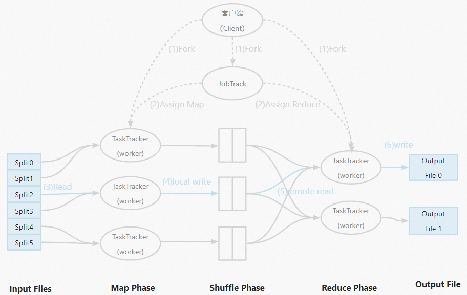
Data skew
Data skew often occurs in the reducer stage. While mappers typically divide input files evenly, data skew occurs when data is unevenly distributed among workers. This uneven distribution causes some workers to finish quickly while others take much longer. In production environments, most data is skewed. This phenomenon follows the Pareto principle, also known as the 80/20 rule. For example, 20% of active users on a forum might contribute 80% of the posts, or 20% of users might generate 80% of the traffic to a website. In the era of big data, data skew can severely impact the performance of distributed programs. A common symptom is a job that appears to be stuck at 99% progress.
How to identify data skew
Procedure
To identify data skew in MaxCompute, use Logview as follows:
In the Fuxi Jobs tab, sort the jobs by Latency in descending order and select the job stage with the longest runtime.
In the Fuxi instance list for that stage, sort the instances by Latency in descending order. Select the instance with a runtime significantly longer than the average (typically the first one on the list). View its output log in the StdOut column.
Use the information in the StdOut log to view the corresponding job execution graph.
Use the key information in the job execution graph to locate the SQL snippet that causes the data skew.
Example
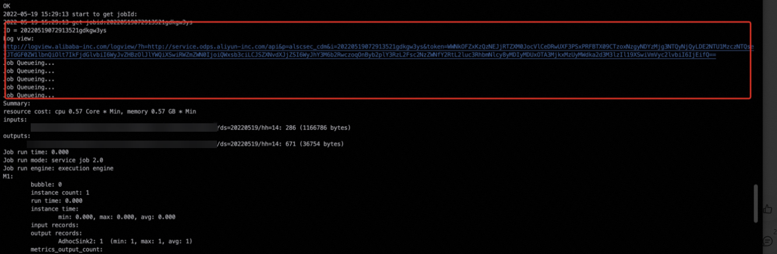
Find the Logview URL in the task's run log. For more information, see Logview entry points.
To quickly pinpoint the issue, sort the Fuxi tasks on the Logview page by Latency in descending order and select the one with the longest runtime.
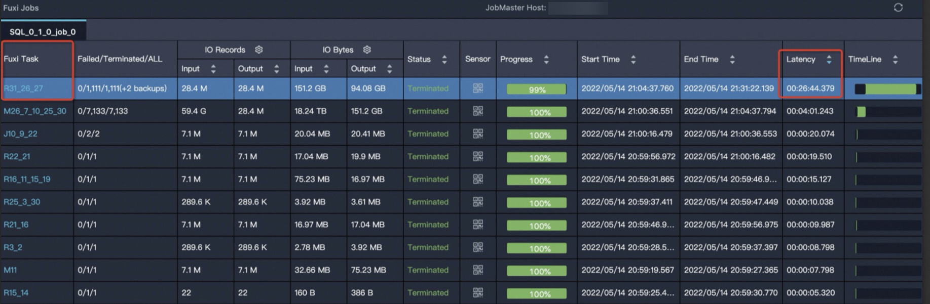
The task
R31_26_27has the longest runtime. Click theR31_26_27task to go to the instance details page, as shown in the following figure.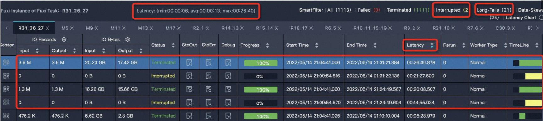 The line
 Latency: {min:00:00:06, avg:00:00:13, max:00:26:40}indicates that the minimum runtime for an instance is6s, the average runtime is13s, and the maximum runtime is26 minutes and 40 seconds.Sort the instances by
Latencyin descending order. You can see that four instances have a long runtime.MaxCompute considers a Fuxi instance a long tail if its runtime is more than twice the average. This means that a task instance with a runtime greater than
26sis identified as a long tail. In this case, 21 instances have runtimes longer than26s. However, the presence of long tail instances does not necessarily indicate data skew. You also need to compare theavgandmaxvalues of the instance runtime. A task is considered to have severe data skew and requires optimization if itsmaxvalue is much greater than itsavgvalue.Click the
 icon in the StdOut column to view the output log, as shown in the following example.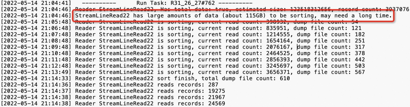
After you pinpoint the issue, go to the Job Details tab, right-click
R31_26_27, and then select Expand All to expand the task. For more information, see Use Logview 2.0 to view job information.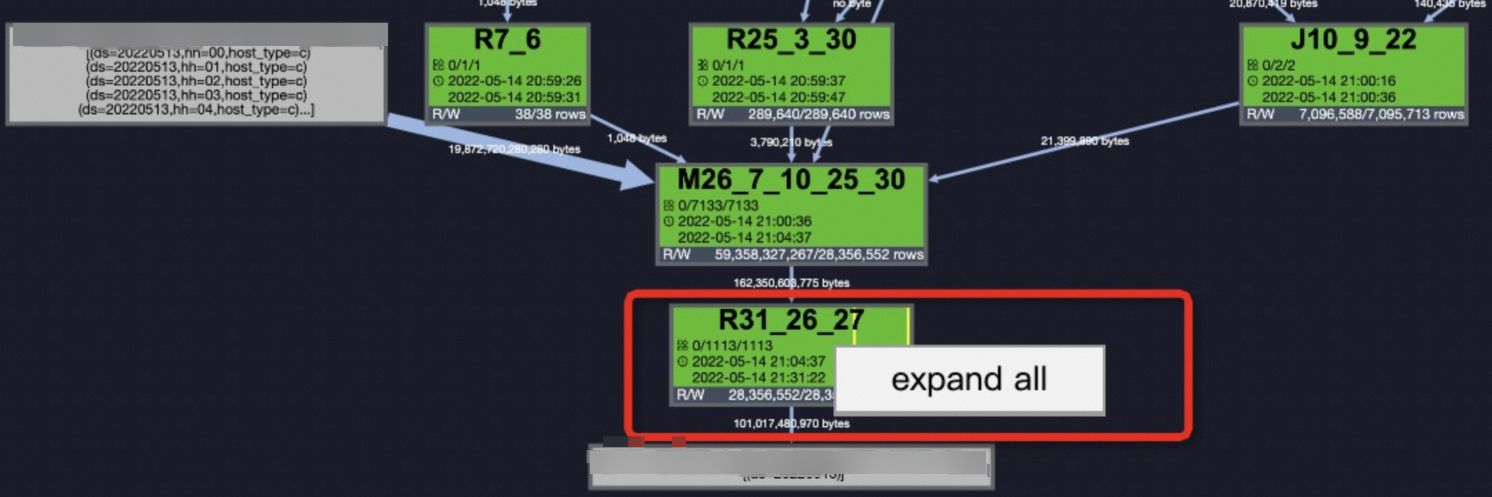 Check the step before
 StreamLineRead22, which isStreamLineWriter21. This allows you to identify the skewed keys (new_uri_path_structure,cookie_x5check_userid, andcookie_userid) and locate the SQL snippet that causes the data skew.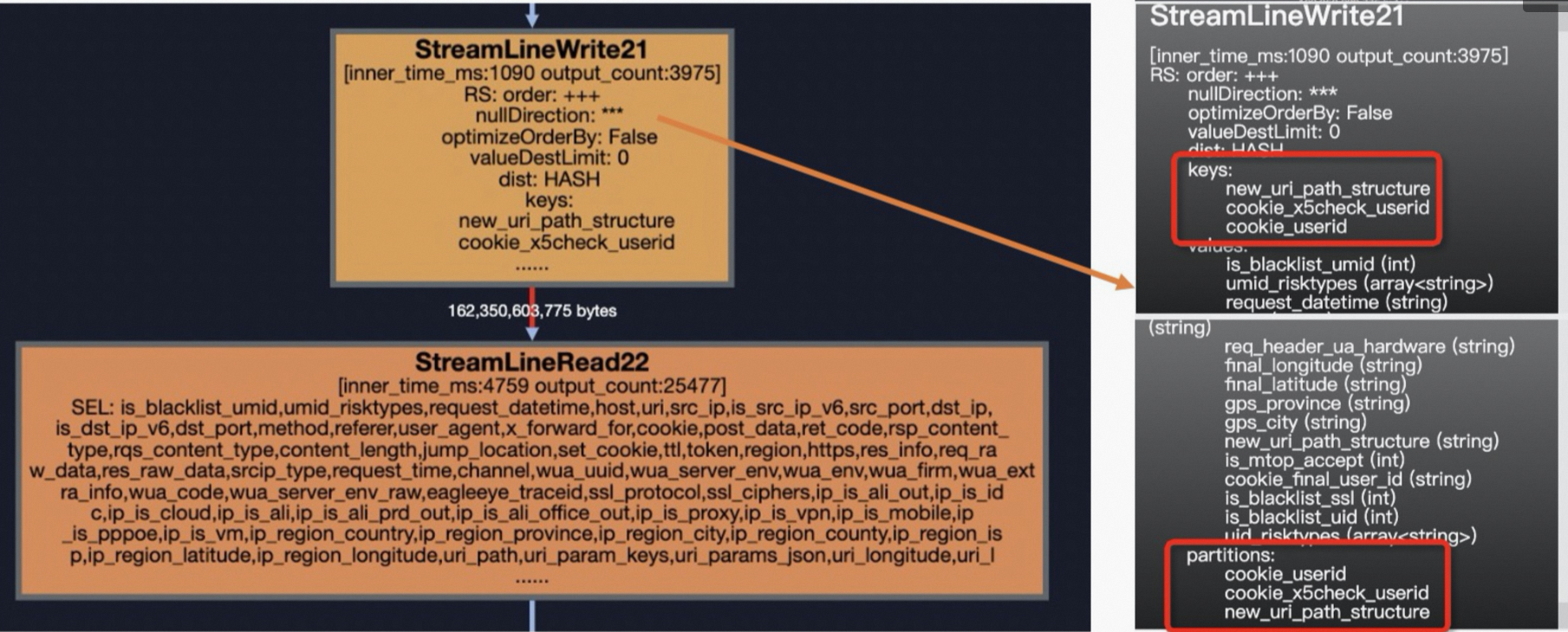
Troubleshooting and resolving data skew
The most common causes of data skew are listed below in descending order of frequency:
JOIN
GROUP BY
COUNT(DISTINCT)
ROW_NUMBER (TopN)
dynamic partition
JOIN
Data skew that occurs in a JOIN operation can be caused by different scenarios, such as joining a large table with a small table, a large table with a medium table, or hot keys that cause long tails.
Large and small tables
Data skew example
In the following example,
t1is a large table, andt2andt3are small tables.SELECT t1.ip ,t1.is_anon ,t1.user_id ,t1.user_agent ,t1.referer ,t2.ssl_ciphers ,t3.shop_province_name ,t3.shop_city_name FROM <viewtable> t1 LEFT OUTER JOIN <other_viewtable> t2 ON t1.header_eagleeye_traceid = t2.eagleeye_traceid LEFT OUTER JOIN ( SELECT shop_id ,city_name AS shop_city_name ,province_name AS shop_province_name FROM <tenanttable> WHERE ds = MAX_PT('<tenanttable>') AND is_valid = 1 ) t3 ON t1.shopid = t3.shop_idSolution
Use the MAPJOIN hint syntax, as shown in the following code.
SELECT  /*+ mapjoin(t2,t3)*/
        t1.ip
        ,t1.is_anon
        ,t1.user_id
        ,t1.user_agent
        ,t1.referer
        ,t2.ssl_ciphers
        ,t3.shop_province_name
        ,t3.shop_city_name
FROM    <viewtable> t1
LEFT OUTER JOIN (<other_viewtable>) t2
ON t1.header_eagleeye_traceid = t2.eagleeye_traceid
LEFT OUTER JOIN (  SELECT  shop_id
                            ,city_name AS shop_city_name
                            ,province_name AS shop_province_name
                    FROM    <tenanttable>
                    WHERE   ds = MAX_PT('<tenanttable>')
                    AND     is_valid = 1
                ) t3
ON t1.shopid = t3.shop_id
Usage notes
When you reference a small table or subquery, you must use its alias.
A MAPJOIN supports a subquery as the small table.
In a MAPJOIN, you can use non-equi-joins or join multiple conditions with
OR. You can compute a Cartesian product by omitting theONclause and usingmapjoin on 1 = 1. For example:select /*+ mapjoin(a) */ a.id from shop a join table_name b on 1=1;. However, this operation may cause data bloat.In a MAPJOIN, separate multiple small tables with commas (
,), for example,/*+ mapjoin(a,b,c)*/.A MAPJOIN loads all data of the specified tables into memory during the map stage. Therefore, the specified tables must be small. The in-memory size of each table cannot exceed 512 MB. This limit applies to the data size after it is loaded into memory, which can be significantly larger than its compressed storage size. You can increase this memory limit up to 8,192 MB by setting the following parameter:
SET odps.sql.mapjoin.memory.max=2048;Limits on JOIN operations in a MAPJOIN:
For a
LEFT OUTER JOIN, the left table must be the large table.For a
RIGHT OUTER JOIN, the right table must be the large table.FULL OUTER JOINis not supported.For an
INNER JOIN, either the left or right table can be the large table.A MAPJOIN supports a maximum of 128 small tables. If you exceed this limit, a syntax error is reported.
Large and medium tables
Data skew example
In the following example,
t0is a large table andt1is a medium-sized table.SELECT request_datetime ,host ,URI ,eagleeye_traceid FROM <viewtable> t0 LEFT JOIN ( SELECT traceid, eleme_uid, isLogin_is FROM <servicetable> WHERE ds = '${today}' AND hh = '${hour}' ) t1 ON t0.eagleeye_traceid = t1.traceid WHERE ds = '${today}' AND hh = '${hour}'Solution
Use the DISTRIBUTED MAPJOIN hint to resolve the data skew, as shown in the following code.
SELECT  /*+distmapjoin(t1)*/
        request_datetime
        ,host
        ,URI
        ,eagleeye_traceid
FROM <viewtable>
    t0
LEFT JOIN (
    SELECT
    traceid,
    eleme_uid,
    isLogin_is
    FROM <servicetable>
    WHERE ds = '${today}'
    AND     hh = '${hour}'
) t1 ON t0.eagleeye_traceid = t1.traceid
WHERE   ds = '${today}'
AND     hh = '${hour}'
Hot key join
Data skew example
In the following table, the
eleme_uidcolumn contains many hot keys, which can easily cause data skew.SELECT eleme_uid, ... FROM ( SELECT eleme_uid, ... FROM <viewtable> )t1 LEFT JOIN( SELECT eleme_uid, ... FROM <customertable> ) t2 ON t1.eleme_uid = t2.eleme_uid;Solutions
You can resolve this issue by using one of the following three methods.
Method
Name
Description
Method 1
Manually split hot keys
Identify the hot keys, filter them from the main table, and process them with a MAPJOIN. Process the remaining non-hot key records with a MergeJoin. Finally, merge the results of both JOINs.
Method 2
SkewJoin hint
Use the hint
/*+ skewJoin(<table_name>[(<column1_name>[,<column2_name>,...])][((<value11>,<value12>)[,(<value21>,<value22>)...])]*/. Using the SkewJoin hint adds an extra step to find the skewed keys, which increases the query run time. If you already know the skewed keys, you can set the SkewJoin parameters to save time.Method 3
Modulo-equi join
Use a multiplier table to distribute the hot keys.
Manually split hot keys.
After the hot values are identified, records containing them are filtered from the main table for a MapJoin. The remaining records without hot values are processed with a MergeJoin. Finally, the results of the two joins are combined. For details, see the following code example:
SELECT
/*+ MAPJOIN (t2) */
eleme_uid,
...
FROM (
    SELECT
    eleme_uid,
    ...
    FROM <viewtable>
    WHERE eleme_uid = <skewed_value>
)t1
LEFT JOIN(
    SELECT
    eleme_uid,
    ...
    FROM <customertable>
    WHERE eleme_uid = <skewed_value>
)  t2
ON t1.eleme_uid = t2.eleme_uid
UNION ALL
SELECT
eleme_uid,
...
FROM (
    SELECT
    eleme_uid,
    ...
    FROM <viewtable>
    WHERE eleme_uid != <skewed_value>
)t3
LEFT JOIN(
    SELECT
    eleme_uid,
    ...
    FROM <customertable>
    WHERE eleme_uid != <skewed_value>
)  t4
ON t3.eleme_uid = t4.eleme_uid
SkewJoin hint.
In a
SELECTstatement, use the hint/*+ skewJoin(<table_name>[(<column1_name>[,<column2_name>,...])][((<value11>,<value12>)[,(<value21>,<value22>)...])]*/to handle the skew. In this hint,table_nameis the name of the skewed table,column_nameis the name of the skewed column, andvalueis the skewed key value. The following code provides an example.-- Method 1: Hint the table name. Note that you hint the table's alias. SELECT /*+ skewjoin(a) */ * FROM T0 a JOIN T1 b ON a.c0 = b.c0 AND a.c1 = b.c1; -- Method 2: Hint the table name and the columns that you suspect are skewed. For example, columns c0 and c1 in table 'a' have data skew. SELECT /*+ skewjoin(a(c0, c1)) */ * FROM T0 a JOIN T1 b ON a.c0 = b.c0 AND a.c1 = b.c1 AND a.c2 = b.c2; -- Method 3: Hint the table name and columns, and provide the skewed key values. If a key value is of the STRING type, enclose it in quotation marks. For example, the values for (a.c0=1 and a.c1="2") and (a.c0=3 and a.c1="4") are both skewed. SELECT /*+ skewjoin(a(c0, c1)((1, "2"), (3, "4"))) */ * FROM T0 a JOIN T1 b ON a.c0 = b.c0 AND a.c1 = b.c1 AND a.c2 = b.c2;NoteThe SkewJoin hint method that directly specifies values is more efficient than manually splitting hot keys or using the hint without specifying values.
JOIN types supported by the SkewJoin hint:
For an
INNER JOIN, you can hint either table in the join.For a
LEFT JOIN,SEMI JOIN, orANTI JOIN, you can hint only the left table.For a
RIGHT JOIN, you can hint only the right table.FULL JOINdoes not support the SkewJoin hint.
We recommend that you add a hint only to a JOIN that is certain to have data skew, because the hint runs an aggregation, which incurs a cost.
The data types of the join keys on the left side of the hinted JOIN must be the same as the data types of the join keys on the right side. Otherwise, the SkewJoin hint does not take effect. For example, the data type of
a.c0must be the same as that ofb.c0, and the data type ofa.c1must be the same as that ofb.c1. You can use the CAST function in a subquery to ensure that the data types are consistent. The following is an example:CREATE TABLE T0(c0 int, c1 int, c2 int, c3 int); CREATE TABLE T1(c0 string, c1 int, c2 int); -- Method 1: SELECT /*+ skewjoin(a) */ * FROM T0 a JOIN T1 b ON cast(a.c0 AS string) = b.c0 AND a.c1 = b.c1; -- Method 2: SELECT /*+ skewjoin(b) */ * FROM (SELECT cast(a.c0 AS string) AS c00 FROM T0 a) b JOIN T1 c ON b.c00 = c.c0;After you add the SkewJoin hint, the optimizer runs an aggregation to get the top 20 hot keys.
20is the default value, which you can change by usingset odps.optimizer.skew.join.topk.num = xx;.The SkewJoin hint supports hinting only one side of a JOIN.
The hinted JOIN must have a
left_key = right_keycondition. Cartesian product JOINs are not supported.You cannot add a SkewJoin hint to a JOIN that already has a MAPJOIN hint.
Modulo-equi join with a multiplier table.
This approach is logically different from the previous three solutions. It does not use a divide-and-conquer strategy. Instead, it uses a multiplier table that contains a single integer column with values from 1 to N, where N is determined by the degree of skew. This table is used to expand the user behavior table by N times. The subsequent JOIN operation then uses two join keys: the user ID and
number. By adding thenumberjoin condition, the data skew that is caused by distributing data based only on user IDs is reduced to1/Nof its original level. However, a drawback of this approach is that it also inflates the data by N times.SELECT eleme_uid, ... FROM ( SELECT eleme_uid, ... FROM <viewtable> )t1 LEFT JOIN( SELECT /*+mapjoin(<multipletable>)*/ eleme_uid, number ... FROM <customertable> JOIN <multipletable> ) t2 ON t1.eleme_uid = t2.eleme_uid AND mod(t1.<value_col>,10)+1 = t2.number;To address the data bloat, you can limit the expansion to only the hot key records in both tables, leaving other non-hot key records unchanged. First, find the hot key records. Then, process the traffic table and the user behavior table separately by adding a new
eleme_uid_joincolumn. If a user ID is a hot key,CONCATa randomly assigned positive integer to it (for example, from 0 to 1,000). Otherwise, keep the original user ID. When joining the two tables, use theeleme_uid_joincolumn. This both distributes the hot keys to reduce skew and avoids unnecessary expansion of non-hot key records. However, this logic heavily rewrites the original business logic SQL and is therefore not recommended.
GROUP BY
The following code provides a pseudo-code example with a GROUP BY clause.
SELECT  shop_id
        ,sum(is_open) AS open_days
FROM    table_xxx_di
WHERE   dt BETWEEN '${bizdate_365}' AND '${bizdate}'
GROUP BY shop_id;
When data skew occurs, you can use one of the following three solutions:
Method | Name | Description |
Method 1 | Set the anti-skew parameter for GROUP BY | Set |
Method 2 | Add a random number | Split the keys that cause long tails. |
Method 3 | Create a rolling table | Reduce costs and improve efficiency. |
Method 1: Set the anti-skew parameter for GROUP BY.
SET odps.sql.groupby.skewindata=true;Method 2: Add a random number.
This solution rewrites the SQL to add a random number, splitting the keys that cause long tails. This is an effective method for resolving long tails in GROUP BY operations.
For the SQL query
Select Key,Count(*) As Cnt From TableName Group By Key;, without a combiner, the mapper node shuffles data to the reducer node, which then performs the COUNT operation. The corresponding execution plan isM->R.Assuming the long-tail key has been identified, you can re-distribute the work for that key as follows:
-- Assume the long-tail key is KEY001.
SELECT  a.Key
        ,SUM(a.Cnt) AS Cnt
FROM(SELECT  Key
            ,COUNT(*) AS Cnt
            FROM    <TableName>
            GROUP BY Key
            ,CASE WHEN KEY = 'KEY001' THEN Hash(Random()) % 50
             ELSE 0
            END
        ) a
GROUP BY a.Key;
The modified execution plan becomes
M->R->R. Although the number of execution steps increases, the overall runtime may be reduced because the long-tail key is processed in two stages. The resource consumption and time efficiency are similar to Method 1. However, in real-world scenarios, there is often more than one long-tail key. Considering the effort of finding long-tail keys and rewriting SQL, Method 1 is often more cost-effective.Method 3: Create a rolling table.
To reduce costs and improve efficiency, you may need to retrieve data from the past year. For online tasks, reading all partitions from
T-1toT-365each time is a significant waste of resources. Creating a rolling table can reduce the number of partitions read without affecting data retrieval for the past year. The following code provides an example.First, initialize 365 days of merchant business data with a GROUP BY aggregation, mark the data update date, and store it as table
a. Subsequent online tasks can then join theT-2day tableawith thetable_xxx_ditable and perform another GROUP BY. This reduces the number of partitions read daily from 365 to 2. The duplication of the primary keyshop_idis greatly reduced, which also decreases resource consumption.-- Create a rolling table. CREATE TABLE IF NOT EXISTS m_xxx_365_df ( shop_id STRING, last_update_ds STRING, `365d_open_days` BIGINT ) PARTITIONED BY ( ds STRING COMMENT 'Date partition' )LIFECYCLE 7; -- Assume the 365-day period is 2021-05-01 to 2022-05-01. Perform a one-time initialization. INSERT OVERWRITE TABLE m_xxx_365_df PARTITION(ds = '20220501') SELECT shop_id, max(ds) as last_update_ds, sum(is_open) AS `365d_open_days` FROM table_xxx_di WHERE dt BETWEEN '20210501' AND '20220501' GROUP BY shop_id; -- Then, the daily online task to be executed is: INSERT OVERWRITE TABLE m_xxx_365_df PARTITION(ds = '${bizdate}') SELECT aa.shop_id, aa.last_update_ds, `365d_open_days` - COALESCE(is_open, 0) AS `365d_open_days` -- Prevent infinite rolling of open days. FROM ( SELECT shop_id, max(last_update_ds) AS last_update_ds, sum(`365d_open_days`) AS `365d_open_days` FROM ( SELECT shop_id, ds AS last_update_ds, sum(is_open) AS `365d_open_days` FROM table_xxx_di WHERE ds = '${bizdate}' GROUP BY shop_id UNION ALL SELECT shop_id, last_update_ds, `365d_open_days` FROM m_xxx_365_df WHERE dt = '${bizdate_2}' AND last_update_ds >= '${bizdate_365}' -- No GROUP BY needed here if the source is already grouped. ) GROUP BY shop_id ) AS aa LEFT JOIN ( SELECT shop_id, is_open FROM table_xxx_di WHERE ds = '${bizdate_366}' ) AS bb ON aa.shop_id = bb.shop_id;
COUNT(DISTINCT)
Suppose a table has the following data distribution.
ds (partition) | cnt (record count) |
20220416 | 73,025,514 |
20220415 | 2,292,806 |
20220417 | 2,319,160 |
Using the following statement can easily cause data skew:
SELECT  ds
        ,COUNT(DISTINCT shop_id) AS cnt
FROM    demo_data0
GROUP BY ds;
The solutions are as follows:
Method | Name | Description |
Method 1 | Parameter tuning | Set |
Method 2 | Generic two-stage aggregation | Append a random number to the partition field value. |
Method 3 | Two-stage-like aggregation | First, group by the |
Method 1: Parameter tuning.
Set the following parameter:
SET odps.sql.groupby.skewindata=true;Method 2: Generic two-stage aggregation.
If the data in the
shop_idfield is unevenly distributed, Method 1 is not effective. A more generic method is to append a random number to the partition field value.-- Method A: Concatenate a random number. CONCAT(ROUND(RAND(),1)*10,'_', ds) AS rand_ds SELECT SPLIT_PART(rand_ds, '_', 2) AS ds ,COUNT(DISTINCT shop_id) AS id_cnt FROM ( SELECT CONCAT(CAST(FLOOR(RAND() * 10) AS STRING), '_', ds) AS rand_ds ,shop_id FROM demo_data0 ) GROUP BY rand_ds; -- Method B: Add a random number field. ROUND(RAND(),1)*10 AS randint10 SELECT ds ,COUNT(DISTINCT shop_id) AS id_cnt FROM (SELECT ds ,shop_id FROM demo_data0 ) GROUP BY ds, FLOOR(RAND() * 10);Method 3: Two-stage-like aggregation.
If the data for the GROUP BY and DISTINCT fields is evenly distributed, you can optimize the query by first applying GROUP BY to the two grouping fields (ds and shop_id) and then using the
count(distinct)command.SELECT ds ,COUNT(shop_id) AS cnt FROM(SELECT ds ,shop_id FROM demo_data0 GROUP BY ds ,shop_id ) GROUP BY ds;
ROW_NUMBER (TopN)
The following code provides a Top-10 example.
SELECT  main_id
        ,type
FROM    (SELECT  main_id
                 ,type
                 ,ROW_NUMBER() OVER(PARTITION BY main_id ORDER BY type DESC ) rn
            FROM <data_demo2>
        ) A
WHERE   A.rn <= 10;
When data skew occurs, you can resolve it by using one of the following methods:
Method | Name | Description |
Method 1 | SQL-based two-stage aggregation | Add a random column or append a random number and use it as a parameter in the PARTITION BY clause. |
Method 2 | UDAF-based two-stage aggregation | Use a UDAF to optimize the query with a min-heap priority queue. |
Method 1: SQL-based two-stage aggregation.
To distribute the data in each partition group as evenly as possible during the map stage, add a random column and use it as a parameter in the PARTITION BY clause.
-- Method 1: Use modulo on a random number.
SELECT  main_id
        ,type
  FROM  (SELECT  main_id
                 ,type
                 ,ROW_NUMBER() OVER(PARTITION BY main_id ORDER BY type DESC ) rn
            FROM (SELECT  main_id
                          ,type
                        FROM (SELECT  main_id
                                      ,type
                                      ,ROW_NUMBER() OVER(PARTITION BY main_id,src_pt ORDER BY type DESC ) rn
                                 FROM (SELECT  main_id
                                               ,type
                                               ,ceil(110 * rand()) % 11 AS src_pt
                                         FROM  data_demo2
                                      )
                                ) B
                        WHERE   B.rn <= 10
                    )
        ) A
WHERE   A.rn <= 10;
-- Method 2: Use a custom random number.
SELECT  main_id
        ,type
  FROM  (SELECT  main_id
                 ,type
                 ,ROW_NUMBER() OVER(PARTITION BY main_id ORDER BY type DESC ) rn
            FROM (SELECT  main_id
                          ,type
                    FROM(SELECT  main_id
                                 ,type
                                 ,ROW_NUMBER() OVER(PARTITION BY main_id,src_pt ORDER BY type DESC ) rn
                           FROM  (SELECT  main_id
                                          ,type
                                          ,ceil(10 * rand()) AS src_pt
                                          FROM    data_demo2
                                  )
                                ) B
                        WHERE B.rn <= 10
                    )
        ) A
WHERE   A.rn <= 10;
Method 2: UDAF-based two-stage aggregation.
The SQL method can result in verbose code that is difficult to maintain. Alternatively, you can use a UDAF with a min-heap priority queue for optimization. In the
iteratephase, only the Top-N elements are kept, and in themergephase, only N elements are merged. The process is as follows:iterate: Push the first K elements. For elements after K, continuously compare them with the top element of the min-heap and swap elements as needed.merge: After merging two heaps, return the top K elements in place.terminate: Return the heap as an array.In the SQL query, split the array into separate rows.
@annotate('* -> array<string>')
class GetTopN(BaseUDAF):
    def new_buffer(self):
        return [[], None]
    def iterate(self, buffer, order_column_val, k):
        # heapq.heappush(buffer, order_column_val)
        # buffer = [heapq.nlargest(k, buffer), k]
        if not buffer[1]:
            buffer[1] = k
        if len(buffer[0]) < k:
            heapq.heappush(buffer[0], order_column_val)
        else:
            heapq.heappushpop(buffer[0], order_column_val)
    def merge(self, buffer, pbuffer):
        first_buffer, first_k = buffer
        second_buffer, second_k = pbuffer
        k = first_k or second_k
        merged_heap = first_buffer + second_buffer
        merged_heap.sort(reverse=True)
        merged_heap = merged_heap[0: k] if len(merged_heap) > k else merged_heap
        buffer[0] = merged_heap
        buffer[1] = k
    def terminate(self, buffer):
        return buffer[0]

SET odps.sql.python.version=cp37;
SELECT main_id,type_val FROM (
  SELECT  main_id ,get_topn(type, 10) AS type_array
  FROM data_demo2
  GROUP BY main_id
)
LATERAL VIEW EXPLODE(type_array)type_ar AS type_val;
Dynamic partition
A dynamic partition allows you to insert data into a partitioned table by specifying a partition column name in the PARTITION clause without providing a specific value. Instead, the partition value is provided by the corresponding column in the SELECT clause. Therefore, the exact partitions to be created are unknown until the SQL query finishes running and the partition column values are determined. For more information, see Insert or overwrite data into dynamic partitions (DYNAMIC PARTITION). The following code provides an SQL example.
CREATE TABLE total_revenues (revenue bigint) partitioned BY (region string);

INSERT overwrite TABLE total_revenues PARTITION(region)
SELECT total_price AS revenue,region
FROM sale_detail;
Dynamic partitions are used in many scenarios and can easily lead to data skew. When data skew occurs, you can resolve it by using one of the following solutions.
Method | Name | Description |
Method 1 | Parameter configuration | Optimize the query by configuring parameters. |
Method 2 | Pruning optimization | Find partitions with a large number of records, prune them, and then insert them separately. |
Method 1: Parameter configuration.
Dynamic partitioning can place data that meets different conditions into different partitions, which avoids the need for multiple INSERT OVERWRITE statements. This can greatly simplify the code, especially when there are many partitions. However, dynamic partitioning can also lead to an excessive number of small files.
Data skew example
Take the following simple SQL as an example:
INSERT INTO TABLE part_test PARTITION(ds) SELECT * FROM part_test;Assume there are K Map instances and N target partitions.
                            ds=1
cfile1                      ds=2
...             X           ds=3
cfilek                      ...
                            ds=n
In the most extreme case,
K*Nsmall files may be generated. An excessive number of small files can put huge management pressure on the file system. Therefore, MaxCompute handles dynamic partitions by introducing an additional level of reducer tasks. It directs data for the same target partitions to be written by the same (or a few) reducer instances, which avoids creating too many small files. This reducer is always the last task in the job. In MaxCompute, this feature is enabled by default, which means the following parameter is set to true:SET odps.sql.reshuffle.dynamicpt=true;Enabling this feature by default solves the problem of too many small files and prevents tasks from failing due to an excessive number of files generated by a single instance. However, it also introduces a new problem: data skew. Additionally, introducing an extra reducer stage consumes computing resources. Therefore, you must carefully weigh the trade-offs.
Solution
The initial purpose of introducing an extra reducer stage by enabling the
set odps.sql.reshuffle.dynamicpt=true;parameter is to solve the problem of too many small files. However, if the number of target partitions is small and there is no risk of having too many small files, enabling this feature by default not only wastes computing resources but also reduces performance. In this case, disabling this feature by settingset odps.sql.reshuffle.dynamicpt=false;can significantly improve performance. The following code provides an example.INSERT overwrite TABLE ads_tb_cornucopia_pool_d PARTITION (ds, lv, tp) SELECT /*+ mapjoin(t2) */ '20150503' AS ds, t1.lv AS lv, t1.type AS tp FROM (SELECT ... FROM tbbi.ads_tb_cornucopia_user_d WHERE ds = '20150503' AND lv IN ('flat', '3rd') AND tp = 'T' AND pref_cat2_id > 0 ) t1 JOIN (SELECT ... FROM tbbi.ads_tb_cornucopia_auct_d WHERE ds = '20150503' AND tp = 'T' AND is_all = 'N' AND cat2_id > 0 ) t2 ON t1.pref_cat2_id = t2.cat2_id;If the default parameters are used for the preceding code, the total runtime of the job is about 1 hour and 30 minutes. The last reducer stage takes about 1 hour and 20 minutes, which accounts for about
90%of the total runtime. The introduction of an extra reducer stage makes the data distribution of each reducer instance very uneven, which leads to a long tail.
For the preceding example, by analyzing the historical number of dynamic partitions generated, we find that only about two dynamic partitions are generated each day. Therefore, you can safely set
set odps.sql.reshuffle.dynamicpt=false;. The job can then be completed in just 9 minutes. In this case, setting this parameter tofalsecan significantly improve performance and save computing time and resources. This single parameter change provides a significant improvement for minimal effort.This optimization is not only for large, long-running jobs that consume a lot of resources, but also for ordinary, short-running jobs that consume fewer resources. As long as dynamic partitioning is used and the number of dynamic partitions is small, you can set the
odps.sql.reshuffle.dynamicptparameter tofalseto save resources and improve performance.Nodes that meet all the following three conditions can be optimized, regardless of the job's duration:
The job uses dynamic partitions.
The number of dynamic partitions is 50 or less.
The job does not have
set odps.sql.reshuffle.dynamicpt=false;.
The execution time of the last Fuxi instance can be used to determine the urgency of setting this parameter for the node. This is identified by the
diag_levelfield. The rules are as follows:Last_Fuxi_Inst_Timeis greater than 30 minutes:Diag_Level=4 ('Critical').Last_Fuxi_Inst_Timeis between 20 and 30 minutes:Diag_Level=3 ('High').Last_Fuxi_Inst_Timeis between 10 and 20 minutes:Diag_Level=2 ('Medium').Last_Fuxi_Inst_Timeis less than 10 minutes:Diag_Level=1 ('Low').
Method 2: Pruning optimization.
To resolve data skew that already exists in the map stage when inserting data into dynamic partitions, you can find and prune the partitions with many records, then insert them separately. Based on the actual use case, you can modify the parameter configuration of the map stage as follows:
SET odps.sql.mapper.split.size=128;
INSERT OVERWRITE TABLE data_demo3 partition(ds,hh)
SELECT  *
FROM    dwd_alsc_ent_shop_info_hi;
The result shows that a full table scan was performed. To further optimize, you can disable the Reduce job introduced by the system, as follows:
SET odps.sql.reshuffle.dynamicpt=false ;
INSERT OVERWRITE TABLE data_demo3 partition(ds,hh)
SELECT *
FROM dwd_alsc_ent_shop_info_hi;
To resolve data skew in the map stage when inserting data into dynamic partitions, find the partitions with many records, prune them, and insert them separately. The specific steps are as follows:
Use the following command to query for specific partitions with a large number of records.
SELECT  ds
        ,hh
        ,COUNT(*) AS cnt
FROM    dwd_alsc_ent_shop_info_hi
GROUP BY ds
         ,hh
ORDER BY cnt DESC;
Some of the partitions are as follows:
ds
hh
cnt
20200928
17
1052800
20191017
17
1041234
20210928
17
1034332
20190328
17
1000321
20210504
1
19
20191003
20
18
20200522
1
18
20220504
1
18
Filter out the partitions with a large number of records, insert the remaining data, and then separately insert the data for the large-record partitions.
SET odps.sql.reshuffle.dynamicpt=false ;
-- Insert data for partitions that do not have a large number of records.
INSERT OVERWRITE TABLE data_demo3 partition(ds,hh)
SELECT  *
FROM    dwd_alsc_ent_shop_info_hi
WHERE   CONCAT(ds,hh) NOT IN ('2020092817','2019101717','2021092817','2019032817');

-- Insert data for partitions that have a large number of records.
set odps.sql.reshuffle.dynamicpt=false ;
INSERT OVERWRITE TABLE data_demo3 partition(ds,hh)
SELECT  *
FROM    dwd_alsc_ent_shop_info_hi
WHERE   CONCAT(ds,hh) IN ('2020092817','2019101717','2021092817','2019032817');

-- Verify the result.
SELECT  ds
  ,hh,COUNT(*) AS cnt
 FROM dwd_alsc_ent_shop_info_hi
 GROUP BY ds,hh ORDER BY cnt desc;