LindormTSDB includes built-in anomaly detection powered by algorithms developed by DAMO Academy. The anomaly_detect() function runs inside the database and continuously learns the statistical characteristics of your time series—trends, seasonality, and variance—to flag data points that deviate significantly from expected behavior.
Applicable engines and versions
Applicable to LindormTSDB. All versions are supported.
Limitations
anomaly_detect() must be used with the SAMPLE BY clause.
How it works
Each call to anomaly_detect() takes a field column and an algorithm name (or model name when in-database machine learning is enabled). As new data points arrive, the algorithm updates its internal state and decides whether each point is anomalous.
Warmup period: Before reporting any anomalies, the algorithm collects enough data to build a baseline. During warmup, the warmup column returns TRUE and no anomalies are flagged—this is expected behavior, not an error. Results return null during this phase. The required warmup length varies by algorithm:
esd,nsigma: 20 data points by default (configurable viawarmupCount)ttest: 20 data points by defaultistl-esd,istl-nsigma: four full cycles of data
State persistence: By default (adhoc_state=FALSE), the algorithm retains its learned state across queries, making it suitable for continuous streaming detection. Set adhoc_state=TRUE for one-off ad-hoc queries, where the state is discarded after the query completes.
Three usage patterns are supported:
| Pattern | Clause | Nested operators | Examples |
|---|---|---|---|
| Scan every data point | SAMPLE BY 0 | None | Examples 1, 2, 3 |
| Downsample then detect | SAMPLE BY <interval> | MIN, MAX, AVG, COUNT, SUM | Example 4 |
| Apply non-downsampling operators | SAMPLE BY 0 | LATEST, DELTA, RATE | Example 5 |
When using SAMPLE BY <interval>, the interval value cannot be 0.
Choose an algorithm
Each algorithm makes different statistical assumptions. Choose based on the anomaly pattern you expect in your data.
| Algorithm | Best for | Not suitable for |
|---|---|---|
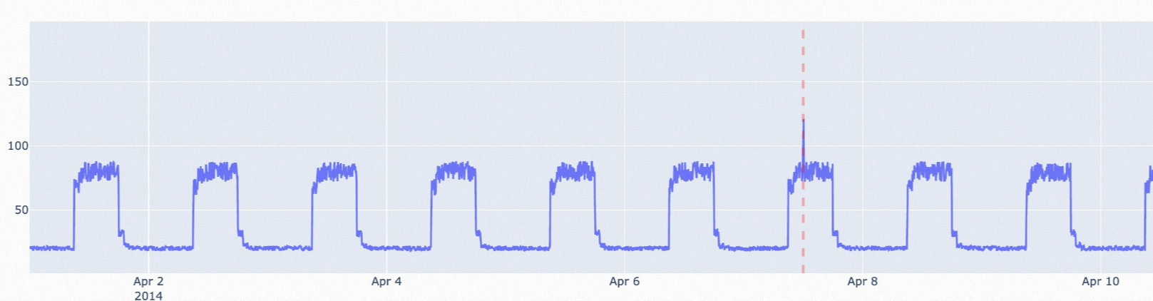
esd | Isolated spikes—a small number of data points with values far outside the norm | Periodic data without first removing seasonality |
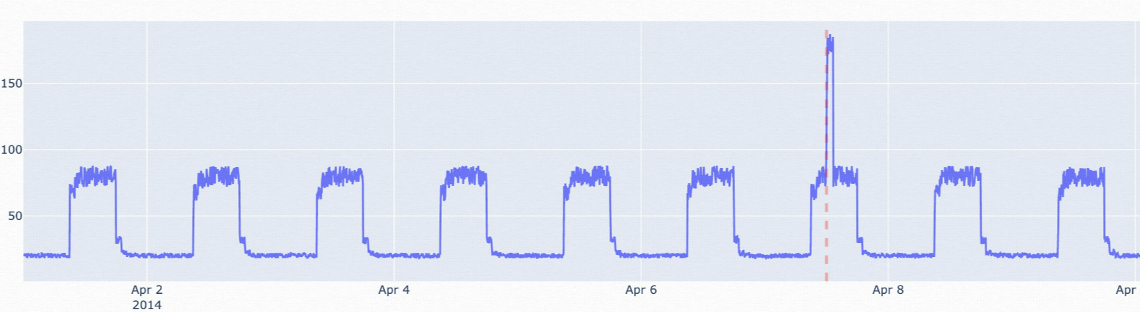
nsigma | Point anomalies where simple root cause analysis matters; data with a stable historical mean | Detecting a small number of extreme spikes (the mean and standard deviation are pulled toward normal values, reducing sensitivity) |
ttest | Detecting shifts in the average value across two consecutive time windows | Single-point spikes |
istl-esd | Periodic data with isolated spikes; removes the seasonal component first, then applies esd to the residual | Non-periodic data |
istl-nsigma | Periodic data where anomalies deviate from the historical average; removes the seasonal component first, then applies nsigma to the residual | Non-periodic data; detecting extreme isolated spikes |
The following figures illustrate typical use cases for each algorithm.
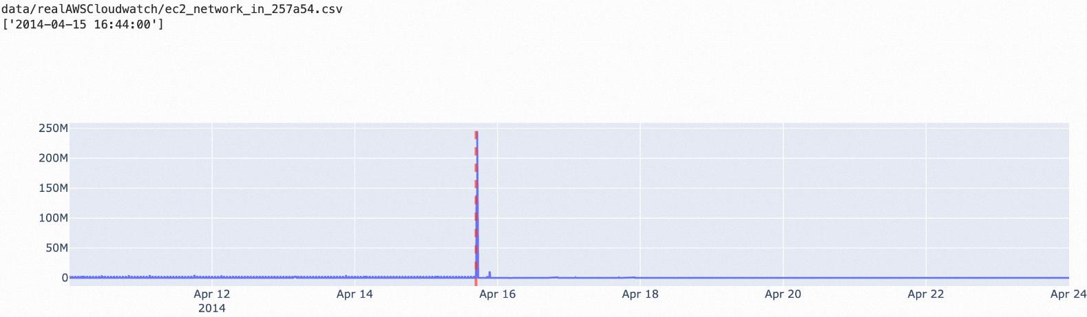
esd: Stable data with a small number of spike outliers.
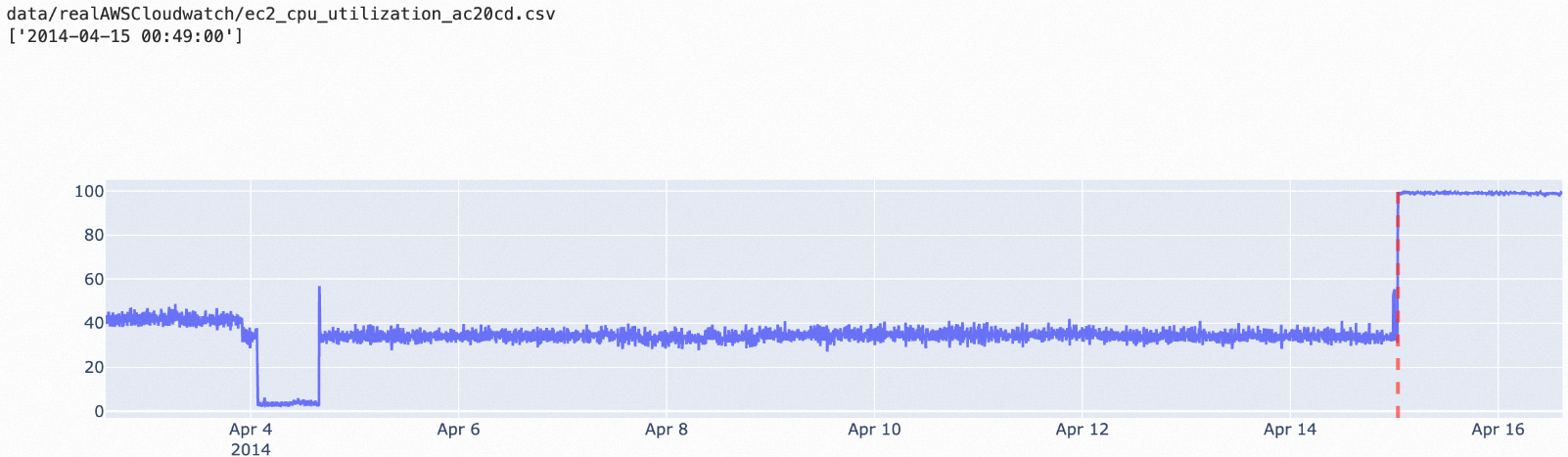
nsigma: Data where anomalous points significantly exceed the historical average. Adjust the
nparameter to control sensitivity.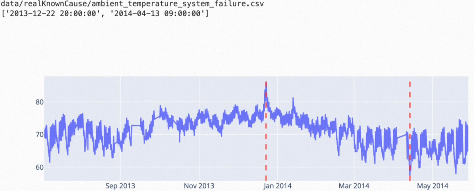
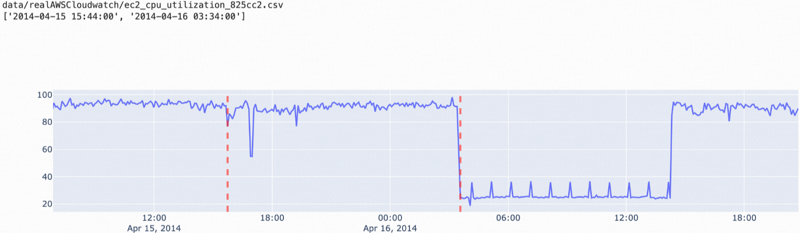
ttest: Data where the average value shifts between two consecutive time windows.
istl-esd: Periodic data with occasional non-periodic spikes.
istl-nsigma: Periodic data with anomalies that deviate from the historical average.
Syntax
SELECT ( select_clause )
FROM table_identifier
WHERE where_clause
SAMPLE BY 0

select_clause  ::= selector [ AS identifier ] ( ',' selector [ AS identifier ] )
selector       ::= tag_identifier
                 | time
                 | anomaly_detect( field_identifier, algo_identifier | model_identifier [, options] )
where_clause   ::= relation ( AND relation )* ( OR relation )*
relation       ::= ( field_identifier | tag_identifier ) operator term
operator       ::= '=' | '<' | '>' | '<=' | '>=' | '!=' | IN | CONTAINS | CONTAINS KEY
anomaly_detect() parameters
| Parameter | Description |
|---|---|
field_identifier | The field column to analyze. Cannot be VARCHAR or BOOLEAN type. |
algo_identifier | The algorithm name. Use when in-database machine learning is not enabled. Valid values: esd, nsigma, ttest, istl-esd, istl-nsigma. |
model_identifier | The model name (VARCHAR type). Use when in-database machine learning is enabled. For details, see In-database machine learning. |
options | Optional. Detection parameters in key=value format, separated by commas. Example: lenDetectWindow=100,adhoc_state=true. |
Parameters
All parameters are specified through the optional options string. Parameters fall into three categories: common, training, and inference.
For guidance on tuning parameters for optimal detection, see Parameter tuning for statistical algorithms and Parameter tuning for decomposition algorithms.
Common parameters
These parameters apply to all algorithms.
| Parameter | Type | Default | Description |
|---|---|---|---|
verbose | BOOLEAN | FALSE | Returns additional diagnostic columns in the result. When TRUE, extra columns are added depending on the algorithm. See Verbose output columns. |
adhoc_state | BOOLEAN | FALSE | Controls whether the algorithm's learned state persists across queries. Set to TRUE for one-off ad-hoc queries (state is discarded after the query). Keep as FALSE for continuous streaming detection (state is retained between queries). For details, see Exception detection status. |
direction | VARCHAR | Up | The direction of deviation to flag as anomalous. Valid values: Up (upward spikes only), Down (downward drops only), Both (both directions). |
Training parameters
Training parameters define the model the algorithm learns during detection. Parameter names are not case-sensitive. Values cannot be NULL and must be within the specified range.
Training parameter values are cleared when LindormTSDB restarts. Reconfigure them after a restart to retrain the model.
| Algorithm | Parameter | Type | Default | Valid values | Description |
|---|---|---|---|---|---|
esd | compression | INTEGER | 100 | (10, 1000) | The space complexity of the data structure. Higher values use more memory but improve accuracy. |
esd | lenHistoryWindow | INTEGER | null | Positive integer >= 20 | The reference window length (number of data points). null uses all data since the first detection. Shorter windows focus on recent data only. |
nsigma | lenHistoryWindow | INTEGER | null | Positive integer >= 20 | The reference window length. Same behavior as esd. |
ttest | lenDetectWindow | INTEGER | 10 | Positive integer | The length of the detection window (the most recent time window to analyze). |
ttest | lenHistoryWindow | INTEGER | 100 | Positive integer >= 20 | The reference window length. Must be larger than lenDetectWindow. |
istl-esd | frequency | VARCHAR | Auto-calculated | Digit + time unit (e.g., 5M, 24H, 1D) | The data collection frequency. If not set, the algorithm infers it—inference may be inaccurate when many values are missing. If set, must match the INTERVAL in SAMPLE BY INTERVAL. |
istl-esd | periods | VARCHAR | Auto-calculated | Digit + time unit (e.g., 5M, 24H, 1D) | The total period length. Specify multiple periods using indexers: periods[0]=1440;periods[1]=1880. |
istl-esd | esd.* | — | — | Same as esd training parameters | Pass esd training parameters with the esd. prefix. Example: esd.lenHistoryWindow=10. |
istl-nsigma | frequency | VARCHAR | Auto-calculated | Same as istl-esd | Same behavior as istl-esd. Must match INTERVAL if set. |
istl-nsigma | periods | VARCHAR | Auto-calculated | Same as istl-esd | Same behavior as istl-esd. |
istl-nsigma | nsigma.* | — | — | Same as nsigma training parameters | Pass nsigma training parameters with the nsigma. prefix. Example: nsigma.lenHistoryWindow=10. |
Supported time units for `frequency` and `periods`:
| Unit | Meaning |
|---|---|
n / ns | Nanosecond |
u / us | Microsecond |
m / ms | Millisecond |
s / S | Second |
M / min | Minute |
H / h | Hour |
D / d | Day |
Inference parameters
Inference parameters affect each detection run and are not case-sensitive.
| Algorithm | Parameter | Type | Default | Valid values | Description |
|---|---|---|---|---|---|
esd | alpha | DOUBLE | 0.1 | (0, 1) | Detection sensitivity. Higher values report more anomalies. |
esd | direction | VARCHAR | Up | Up / Down / Both | The direction of anomalies to detect. |
esd | maxAnomalyRatio | DOUBLE | 0.3 | (0, 1] | The maximum fraction of data points that can be flagged as anomalous. For example, maxAnomalyRatio=0.3 with direction=Up means data points below the 70th percentile are not flagged. Setting to 1 returns no anomalies. |
esd | warmupCount | INTEGER | 20 | Positive integer | The minimum number of data points required before the algorithm starts reporting anomalies. |
nsigma | n | DOUBLE | 3.0 | Non-zero float | The anomaly threshold in standard deviations. Positive: flag when (current - mean) > n x std. Negative: flag when (mean - current) > n x std. |
nsigma | warmupCount | INTEGER | 20 | Positive integer | The minimum number of data points required before reporting anomalies. |
ttest | alpha | DOUBLE | 0.05 | (0, 1) | Detection sensitivity. Higher values report more anomalies. |
ttest | direction | VARCHAR | Up | Up / Down / Both | The direction of anomalies to detect. |
istl-esd | esd.* | — | — | Same as esd inference parameters | Pass esd inference parameters with the esd. prefix. Example: esd.direction=Both. |
istl-nsigma | nsigma.* | — | — | Same as nsigma inference parameters | Pass nsigma inference parameters with the nsigma. prefix. Example: nsigma.n=5. |
Verbose output columns
When verbose=TRUE, additional diagnostic columns appear in the result. The columns vary by algorithm.
nsigma
Same columns as esd, except upperBound, lowerBound, and median are not included. The threshold column represents the judgment threshold for anomalyScore.
istl-esd
| Column | Type | Description |
|---|---|---|
anomaly | BOOLEAN | Whether the data point is anomalous. |
anomalyLevel | STRING | Same as esd. |
residual | DOUBLE | The residual value after removing the trend and seasonal components (original = residual + trend + season). Returns 0 during warmup. |
trend | DOUBLE | The trend component extracted from the original data. Returns 0 during warmup. |
season | DOUBLE | The seasonal component extracted from the original data. Returns 0 during warmup. |
warmup | BOOLEAN | TRUE: algorithm is initializing (requires four full cycles). During warmup, residual, trend, and season values are invalid (0). FALSE: algorithm is ready. |
Additional esd and ttest columns | — | Returned when esd.verbose=true. Includes all esd and ttest verbose columns except anomaly, warmup, and anomalyLevel. |
istl-nsigma
Same structure as istl-esd, using nsigma columns instead. Enable with nsigma.verbose=true.
Examples
All examples use the sensor table with the following schema:
| Column | Type | Role |
|---|---|---|
device_id | tag | Device identifier |
region | tag | Geographic region |
time | — | Timestamp |
temperature | field | Measurement value |
Example 1: Detect anomalies across all devices (esd)
SELECT device_id, region, time, anomaly_detect(temperature, 'esd') AS detect_result
FROM sensor
WHERE time >= '2022-01-01 00:00:00' AND time < '2022-01-01 00:01:00'
SAMPLE BY 0;
The query scans every data point in the specified time range and returns a boolean result per point. A value of true means the algorithm flagged that point as anomalous.
+-----------+----------+---------------------------+---------------+
| device_id |  region  |           time            | detect_result |
+-----------+----------+---------------------------+---------------+
| F07A1260  | north-cn | 2022-01-01T00:00:00+08:00 | true          |
| F07A1260  | north-cn | 2022-01-01T00:00:01+08:00 | false         |
| F07A1260  | north-cn | 2022-01-01T00:00:02+08:00 | true          |
| F07A1261  | south-cn | 2022-01-01T00:00:00+08:00 | false         |
| F07A1261  | south-cn | 2022-01-01T00:00:01+08:00 | false         |
| F07A1261  | south-cn | 2022-01-01T00:00:02+08:00 | false         |
| F07A1261  | south-cn | 2022-01-01T00:00:03+08:00 | false         |
+-----------+----------+---------------------------+---------------+
Example 2: Filter by device before detection (esd)
SELECT device_id, region, time, anomaly_detect(temperature, 'esd') AS detect_result
FROM sensor
WHERE device_id IN ('F07A1260') AND time >= '2022-01-01 00:00:00' AND time < '2022-01-01 00:01:00'
SAMPLE BY 0;
+-----------+----------+---------------------------+---------------+
| device_id | region | time | detect_result |
+-----------+----------+---------------------------+---------------+
| F07A1260 | north-cn | 2022-01-01T00:00:00+08:00 | true |
| F07A1260 | north-cn | 2022-01-01T00:00:01+08:00 | false |
| F07A1260 | north-cn | 2022-01-01T00:00:02+08:00 | true |
+-----------+----------+---------------------------+---------------+Example 3: Tune detection parameters (esd)
Pass detection parameters as a comma-separated key=value string to adjust sensitivity.
SELECT device_id, region, time,
       anomaly_detect(temperature, 'esd', 'lenHistoryWindow=30,maxAnomalyRatio=0.1') AS detect_result
FROM sensor
WHERE device_id IN ('F07A1260') AND time >= '2022-01-01 00:00:00' AND time < '2022-01-01 00:01:00'
SAMPLE BY 0;
+-----------+----------+---------------------------+---------------+
| device_id | region | time | detect_result |
+-----------+----------+---------------------------+---------------+
| F07A1260 | north-cn | 2022-01-01T00:00:00+08:00 | false |
| F07A1260 | north-cn | 2022-01-01T00:00:01+08:00 | false |
| F07A1260 | north-cn | 2022-01-01T00:00:02+08:00 | true |
+-----------+----------+---------------------------+---------------+Example 4: Downsample before detection (MAX, 1-minute interval)
Use a downsampling operator inside anomaly_detect() together with SAMPLE BY <interval>.
SELECT time, anomaly_detect(max(temperature), 'esd') AS ad_result, max(temperature) AS rawVal
FROM sensor
SAMPLE BY 1m;
+---------------------------+-----------+-------------+
| time | ad_result | rawVal |
+---------------------------+-----------+-------------+
| 2022-04-12T06:00:00+08:00 | null | 923091.3175 |
| 2022-04-11T08:00:00+08:00 | null | 8035700 |
| 2022-04-11T09:00:00+08:00 | null | 8035690.25 |
| 2022-04-11T10:00:00+08:00 | null | 3306277.545 |
| 2022-04-11T11:00:00+08:00 | null | 5921167.787 |
| 2022-04-11T12:00:00+08:00 | null | 833541.304 |
+---------------------------+-----------+-------------+ad_result is null because the algorithm is still in the warmup phase (insufficient data points collected).
Example 5: Apply a non-downsampling operator (LATEST)
Use SAMPLE BY 0 with operators like LATEST, DELTA, or RATE.
SELECT time, anomaly_detect(latest(temperature), 'esd') AS ad_result, latest(temperature) AS latestVal
FROM sensor
SAMPLE BY 0;
+---------------------------+-----------+-------------+
| time | ad_result | latestVal |
+---------------------------+-----------+-------------+
| 2022-04-12T06:00:00+08:00 | false | 923091.3175 |
| 2022-04-13T07:00:00+08:00 | false | 8037506.75 |
| 2022-04-13T07:00:00+08:00 | false | 50490.2 |
+---------------------------+-----------+-------------+